Models are about what changes, and what doesn't
How do you build a model from first principles? Here is a step by step guide.
Following on from last week’s post on Principled Bayesian Workflow I want to reflect on how to motivate a model.
The purpose of most models is to understand change, and yet, considering what doesn’t change and should be kept constant can be equally important.
I will go through a couple of models in this post to illustrate this idea. The purpose of the model I want to build today is to predict how much ice cream is sold for different temperatures \((t)\). I am interested in the expected sales \((\mu(t))\), but also the data generating distribution that behaves in line with the observations \((y(t))\) and helps me to understand the variance of my sales.
Data
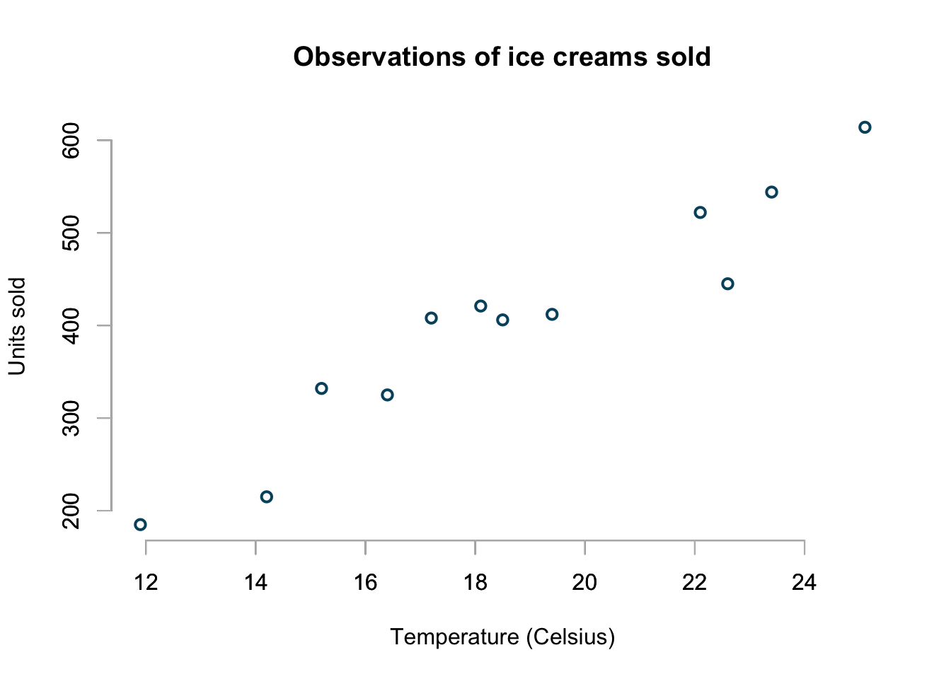
My data set is quite small, it contains the units of ice cream sold for 12 different temperatures from \(11.9^\circ C\) to \(25.1^\circ C\).
icecream <- data.frame(
  temp=c(11.9, 14.2, 15.2, 16.4, 17.2, 18.1,
         18.5, 19.4, 22.1, 22.6, 23.4, 25.1),
  units=c(185L, 215L, 332L, 325L, 408L, 421L,
          406L, 412L, 522L, 445L, 544L, 614L)
  )
This is the same data set I used earlier to discuss generalised linear models (GLMs.)
Model building
Models are about what changes, and what doesn’t. Some are useful.
In mathematics change is often best described with differential equations, and that’s how I will motivate and justify my models today.
If something doesn’t change, we shouldn’t expected a variation of its measurement, and hence, constant variance \((\sigma^2)\) becomes a natural choice. The same can be said, if the change is constant.
No change
The simplest model is to assume no change. Hot or cold, we assume to sale the same amount of ice cream. I can express this as an ordinary differential equation (ODE):
\[ \frac{d\mu(t)}{dt} = 0,\quad\mu(0) = \mu_0 \] It’s solution is \(\mu(t) = \mu_0\) and hence, we could assume for the observable data \(y(t)\): \[ y(t) \sim \mathcal{N}(\mu_0, \sigma^2) \]
Of course, this can’t be right. I would expect higher sales of ice cream for higher temperatures.
Constant change
By assuming constant change I mean that the increase in sales is constant, regardless of the starting temperature, i.e. a change in temperature from \(7^\circ C\) to \(12^\circ C\) will cause the same increase in sales as from \(22^\circ C\) to \(27^\circ C\), or to put this into a ODE:
\[ \frac{d\mu(t)}{dt} = b,\quad \mu(0)=a \] Solving the ODE gives us the classic linear equation for the mean: \[ \mu(t) = a + b\,t \] Now, as we are assuming constant change, I should also assume that the variance \((\sigma^2)\) around my data doesn’t change either and hence, I could model my data as Gaussian again:
\[ y(t) \sim \mathcal{N}(\mu(t), \sigma^2) = \mathcal{N}(a + b\,t, \sigma^2) \]
This model makes a little more sense, but it could also predict negative expected sales, if \(a\) is negative. In addition, generating data from this distribution will produce negative values occasional as well, even if \(a>0\).
Constant sales growth rate
Assuming a constant sales growth rate means that a \(1^\circ C\) increase in temperature is responded by the same proportional change in sales, i.e. for every \(1^\circ C\) increase the sales would increase by \(b\)%. Thus, we are moving from an additive to a multiplicative scale. We can describe the change in the median sales as: \[ \frac{d\mu(t)}{dt} = \mu(t) \, b,\quad \mu(0)=a \] The solution to this ODE is exponential growth (\(b>0\)), or decay (\(b<0\)): \[ \mu(t) = a \, \exp(b\,t) \] On a log-scale we have: \[ \log{\mu(t)} = \log{a} + b\,t \]
This is a linear model again. Thus, we can assume constant change and variance \((\sigma^2)\) on a log-scale. A natural choice for the data generating distribution would be:
\[ \log{y}(t) \sim \mathcal{N}(\log{a} + b\,t, \sigma^2) \]
Or, in other words, I believe the data follows a log-normal distribution. The expected sale for a given temperature is \(E[y(t)]=\exp{(\mu(t)+\sigma^2/2)}\), its median is \(\exp{(\mu(t))}\). In addition this also means that we assume a constant coefficient of variation \((CV)\) on the original scale:
\[ \begin{aligned} CV &=\frac{\sqrt{Var[y]}}{E[y]} \\ & = \frac{\sqrt{(e^{\sigma^2} - 1)e^{2\mu(t)+\sigma^2}}}{e^{\mu(t)+\sigma^2/2}} \\ & = \sqrt{e^{\sigma^2} - 1} \\ & = const \end{aligned} \]
Although this model avoids negative sales, it does assume exponential growth as temperatures increase. Perhaps, this a little too optimistic.
Constant demand elasticity
A constant demand elasticity of \(b = 60\)% would mean in this context that a 10% increase in the temperature would lead to a 6% increase in demand/ sales.
Thus, the relative change in sales is proportional to the relative change in temperature:
\[ {\frac{d\mu(t)}{\mu(t)}} = b {\frac{dt}{t}} \] Re-arranging and adding an initial value gives us the following ODE:
\[ \frac{d\mu(t)}{dt} = \frac{b}{t}\mu(t),\quad\mu(1)=a \]
It’s solution is:
\[ \mu(t) = \exp{(a + b \log(t))} = \exp{(a)} \cdot t^b \]
Now take the log on both sides and we are back to linear regression equation:
\[\log(\mu(t)) = a + b \log(t)\] Thus, we are assuming constant change on a log-log scale. We can assume a log-normal data generating distribution again, but this time we measure temperature on a log-scale as well.
\[ \log{y(t)} \sim \mathcal{N}(a + b\log{t}, \sigma^2) \]
This model, as well as the log-transformed model above, predicts ever increasing ice cream sales as temperature rises.
Constant market size
However, if I believe that my market/ sales opportunities are limited, i.e. we reach market saturation, then a logistic growth model would make more sense.
Let’s assume as temperature rises, sales will increase exponential initially and then tail off to a saturation level \(M\). The following ODE would describe this behaviour:
\[ \frac{d\mu(t)}{dt} = b\, \mu(t) (1 - \mu(t)/M),\quad\mu(0)=\mu_0 \]
Integrating the ODE provides us with the logistic growth curve (often used to describe population growth):
\[ \mu(t) = \frac{ M }{1 + \frac{M-\mu_0}{\mu_0}e^{-b\,t}} = \frac{\mu_0 M e^{b\,t}}{\mu_0 (e^{b\,t} - 1) + M} \]
Setting \(M=1\) gives me the proportion of maximum sales, and setting \(a:=(1-\mu_0)/\mu_0\) gives us:
\[ \begin{aligned} \mu_p(t) &= \frac{ 1 }{1 + \frac{1-\mu_0}{\mu_0}e^{-b\,t}} \\ & = \frac{1}{1 + e^{-(a+b\,t)}} \end{aligned} \]
Nice, this is logistic regression. Defining \(\mbox{logistic}(u) := \frac{1}{1 + e^{-u}}\), we can see that the above has a linear expression in \(u\).
Thus, if I set \(z(t):=y(t)/M\), I could assume the Binomial distribution as the data generating process:
\[ z(t) \sim \mbox{Bin}\left(M, \mbox{logistic}(\mu_p(t))\right) \]
But I don’t know \(M\). Thus, I have to provide a prior distribution, for example a Poisson distribution with parameter (my initial guess) \(M_0\)
\[ M \sim \mbox{Pois}(M_0) \]
Or, alternatively I could consider the Poisson distribution as the data generating distribution, with its mean and variance being described by the non-linear growth curve above (this is not a GLM, unlike the models so far):
\[ y(t) \sim \mbox{Pois}(\mu(t)) = \mbox{Pois}\left(\frac{\mu_0 M e^{b\,t}}{\mu_0 (e^{b\,t} - 1) + M}\right) \]
The Poisson distribution has the property that the mean and variance are the same. If \(y \sim \mbox{Pois}(\lambda)\), then \(E[y] =\mbox{Var}[y] = \lambda\), but more importantly, we are generating integers, in line with the observations.
So, let’s generate some data to check if this approach makes sense in the temperature range from \(-5^\circ C\) to \(35^\circ C\).
Let’s put priors over the parameters: \[ \begin{aligned} \mu_0 &\sim \mathcal{N}(10, 1),\quad \mbox{ice creams sold at }0^\circ C\\ b & \sim \mathcal{N}(0.2, 0.02^2),\quad \mbox{inital growth rate} \\ M & \sim \mathcal{N}(800, 40^2) ,\quad \mbox{total market size} \end{aligned} \]
temperature <- c(-5:35)
n <- length(temperature)
nSim <- 10000
set.seed(1234)
# Priors
mu0 = rep(rnorm(nSim, 10, 1), each=n)
b = rep(rnorm(nSim, 0.2, 0.02), each=n)
M = rep(rnorm(nSim, 800, 40), each=n)
lambda = matrix(M/(1 + (M - mu0)/mu0 * exp(-b * rep(temperature, nSim))),
                ncol=n)
With those preparations done I can simulate data:
y_hat_p <- matrix(rpois(nSim*n, lambda), nrow=n)
probs <- c(0.025, 0.25, 0.5, 0.75, 0.975)
pp=t(apply(y_hat_p, 1, quantile, probs=probs))
matplot(temperature, pp, t="l", bty="n",
        main=paste("Poisson percentiles:",
                   "2.5%, 25%, 50%, 75%, 97.5%", sep="\n"))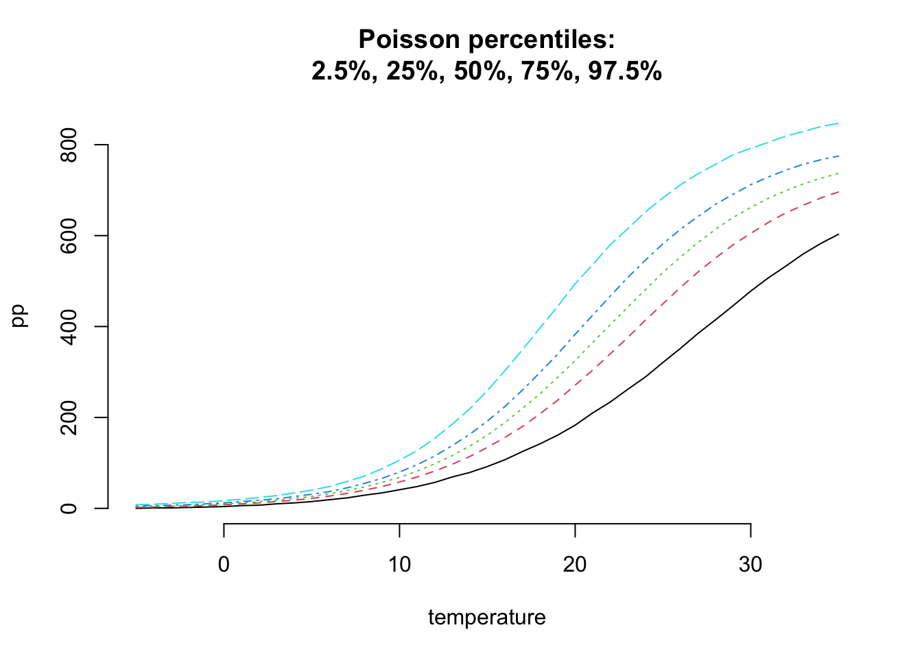
This looks reasonable, but the interquartile range looks quite narrow.
Hence, I want to consider the Negative-Binomial distribution, which has an additional shape parameter \(\theta\) to allow for over-dispersion, i.e. the variance can be greater than the mean. A Negative Binomial distribution with parameters \(\mu\) and \(\theta\) has mean \(\mu\) and variance \(\mu + \mu^2/\theta\). With \(\theta \to \infty\) we are back to a Poisson distribution.
library(MASS) # provides negative binomial
y_hat_nb <- matrix(rnegbin(nSim*n, lambda, theta=20), nrow=n)
nbp <- t(apply(y_hat_nb, 1, quantile, probs=probs))
matplot(temperature, nbp, t="l", bty="n",
        main=paste("Negative Binomial percentiles:",
        "2.5%, 25%, 50%, 75%, 97.5%", sep="\n"))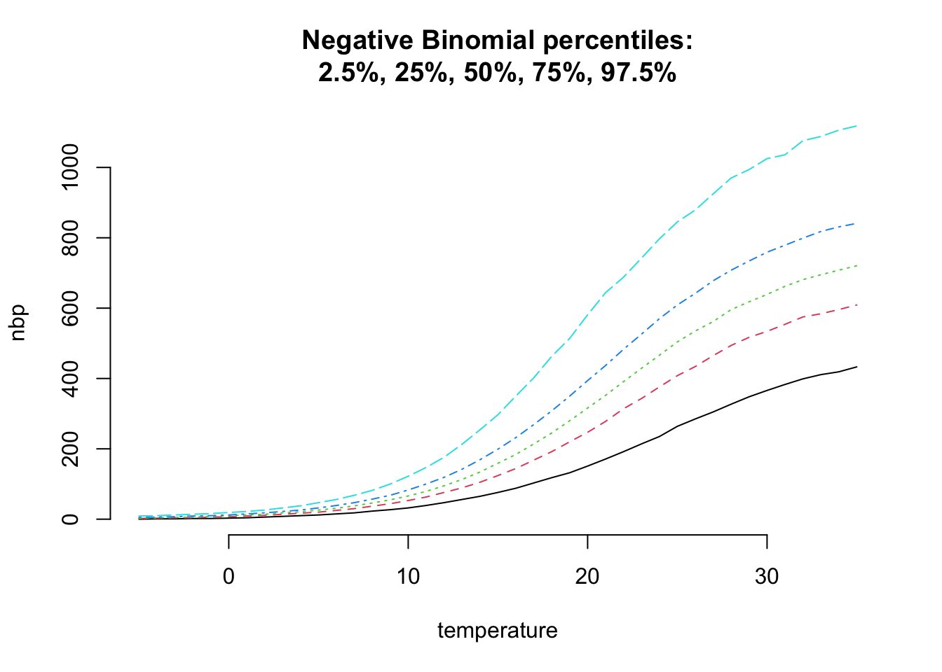
This looks a little more realistic and adds more flexibility to my model.
Finally, I am getting to a stage where it makes sense to make use of my data.
Fitting the model
Using brms I can fit the non-linear logistic growth curve with
a Negative-Binomial data generating distribution.
Note, I put lower bounds on the prior parameter distributions at \(0\), as I allow for high variances and negative values don’t make sense for them.
library(rstan)
rstan_options(auto_write = TRUE)
options(mc.cores = parallel::detectCores())
library(brms)
mdl <- brm(bf(units ~ M  / (1 + (M - mu0) / mu0 * exp( -b * temp)),
              mu0 ~ 1,
              b ~ 1,
              M ~ 1,
              nl = TRUE),
           data = icecream,
           family = brmsfamily("negbinomial", "identity"),
           prior = c(prior(normal(10, 100), nlpar = "mu0", lb=0),
                     prior(normal(0.2, 1), nlpar = "b", lb=0),
                     prior(normal(800, 400), nlpar = "M", lb=0)),
seed = 1234, control = list(adapt_delta=0.9))mdl## Family: negbinomial
## Links: mu = identity; shape = identity
## Formula: units ~ M/(1 + (M - mu0)/mu0 * exp(-b * temp))
## mu0 ~ 1
## b ~ 1
## M ~ 1
## Data: icecream (Number of observations: 12)
## Draws: 4 chains, each with iter = 2000; warmup = 1000; thin = 1;
## total post-warmup draws = 4000
##
## Population-Level Effects:
## Estimate Est.Error l-95% CI u-95% CI Rhat Bulk_ESS Tail_ESS
## mu0_Intercept 35.15 20.32 6.64 80.94 1.00 996 1303
## b_Intercept 0.18 0.05 0.11 0.30 1.00 952 1225
## M_Intercept 809.08 225.05 540.58 1381.66 1.00 1040 1459
##
## Family Specific Parameters:
## Estimate Est.Error l-95% CI u-95% CI Rhat Bulk_ESS Tail_ESS
## shape 92.80 52.89 27.60 231.96 1.00 1148 1683
##
## Draws were sampled using sampling(NUTS). For each parameter, Bulk_ESS
## and Tail_ESS are effective sample size measures, and Rhat is the potential
## scale reduction factor on split chains (at convergence, Rhat = 1).plot(mdl)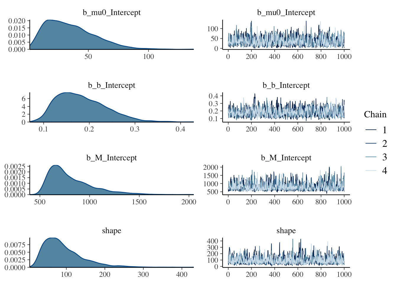
The output looks reasonably well behaved. The estimated standard error for \(\mu_0\) is high, and the 95% credible interval is also quite wide. But I have to remember, the parameter describes the average number of ice cream sold at \(0^\circ C\) and the lowest data point we have for that is only at \(11.9^\circ C\).
Indeed, I have only 12 data points, so not too surprising the credible interval around \(M\), the total market size, is quite wide too. But like for the other parameters, its posterior standard error has shrunk considerably from the one assumed in the prior parameter distribution.
Let’s review the posterior predictive distribution for temperatures from \(-5^\circ C\) to \(35^\circ C\):
pp <- brms::posterior_predict(mdl, newdata=data.frame(temp=temperature))
pp_probs <- t(apply(pp, 2, quantile, probs=probs))
matplot(temperature, pp_probs, t="l", bty="n",
        main=paste("Posterior predictive percentiles:",
                   "2.5%, 25%, 50%, 75%, 97.5%", sep="\n"),
        ylab="Units of icecream sold",
        xlab="Temperature")
points(icecream$temp, icecream$units, pch=19)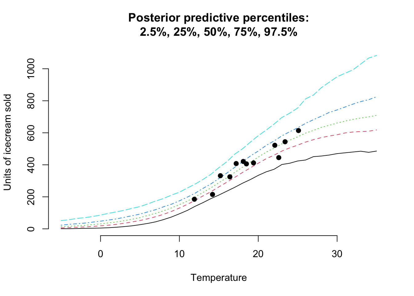
Hurray! This looks really good.
I am happy with the model and its narrative. The parameters are easy interpretable, the curve can be explained and the model generates positive integers, in-line with the data.
Of course, there will be many other factors that influence the sales of ice cream, but I am confident that the temperature is the main driver.
Conclusion
Approaching the model build by thinking about how the sale of ice cream will change, as the temperature changes, and considering what to keep constant has led me down the road of differential equations.
With a small data set like this, starting from a simple model and reasoning any additional complexity has helped me to develop a better understanding of what a reasonable underlying data generating process might be.
Indeed, generating data from the model before using the data, helped to check my understanding of how the model might perform.
Thanks to Stan and brms, I was freed from the constrains under GLMs and I could select my own non-linear model for the expected sales and distribution family.
Session Info
sessionInfo()## R version 4.2.0 (2022-04-22)
## Platform: aarch64-apple-darwin20 (64-bit)
## Running under: macOS Monterey 12.4
##
## Matrix products: default
## BLAS: /Library/Frameworks/R.framework/Versions/4.2-arm64/Resources/lib/libRblas.0.dylib
## LAPACK: /Library/Frameworks/R.framework/Versions/4.2-arm64/Resources/lib/libRlapack.dylib
##
## locale:
## [1] en_US.UTF-8/en_US.UTF-8/en_US.UTF-8/C/en_US.UTF-8/en_US.UTF-8
##
## attached base packages:
## [1] stats graphics grDevices utils datasets methods base
##
## other attached packages:
## [1] brms_2.17.0 Rcpp_1.0.8.3 rstan_2.21.5
## [4] ggplot2_3.3.6 StanHeaders_2.21.0-7 MASS_7.3-57
##
## loaded via a namespace (and not attached):
## [1] minqa_1.2.4 TH.data_1.1-1 colorspace_2.0-3
## [4] ellipsis_0.3.2 ggridges_0.5.3 estimability_1.3
## [7] markdown_1.1 base64enc_0.1-3 rstudioapi_0.13
## [10] farver_2.1.0 DT_0.23 fansi_1.0.3
## [13] mvtnorm_1.1-3 bridgesampling_1.1-2 codetools_0.2-18
## [16] splines_4.2.0 knitr_1.39 shinythemes_1.2.0
## [19] bayesplot_1.9.0 projpred_2.1.1 jsonlite_1.8.0
## [22] nloptr_2.0.0 shiny_1.7.1 compiler_4.2.0
## [25] emmeans_1.7.3 backports_1.4.1 assertthat_0.2.1
## [28] Matrix_1.4-1 fastmap_1.1.0 cli_3.3.0
## [31] later_1.3.0 htmltools_0.5.2 prettyunits_1.1.1
## [34] tools_4.2.0 igraph_1.3.1 coda_0.19-4
## [37] gtable_0.3.0 glue_1.6.2 reshape2_1.4.4
## [40] dplyr_1.0.9 posterior_1.2.1 jquerylib_0.1.4
## [43] vctrs_0.4.1 nlme_3.1-157 blogdown_1.10
## [46] crosstalk_1.2.0 tensorA_0.36.2 xfun_0.31
## [49] stringr_1.4.0 ps_1.7.0 lme4_1.1-29
## [52] mime_0.12 miniUI_0.1.1.1 lifecycle_1.0.1
## [55] gtools_3.9.2 zoo_1.8-10 scales_1.2.0
## [58] colourpicker_1.1.1 promises_1.2.0.1 Brobdingnag_1.2-7
## [61] parallel_4.2.0 sandwich_3.0-1 inline_0.3.19
## [64] shinystan_2.6.0 gamm4_0.2-6 yaml_2.3.5
## [67] gridExtra_2.3 loo_2.5.1 sass_0.4.1
## [70] stringi_1.7.6 highr_0.9 dygraphs_1.1.1.6
## [73] checkmate_2.1.0 boot_1.3-28 pkgbuild_1.3.1
## [76] rlang_1.0.2 pkgconfig_2.0.3 matrixStats_0.62.0
## [79] distributional_0.3.0 evaluate_0.15 lattice_0.20-45
## [82] purrr_0.3.4 labeling_0.4.2 rstantools_2.2.0
## [85] htmlwidgets_1.5.4 processx_3.5.3 tidyselect_1.1.2
## [88] plyr_1.8.7 magrittr_2.0.3 bookdown_0.26
## [91] R6_2.5.1 generics_0.1.2 multcomp_1.4-19
## [94] DBI_1.1.2 mgcv_1.8-40 pillar_1.7.0
## [97] withr_2.5.0 xts_0.12.1 survival_3.3-1
## [100] abind_1.4-5 tibble_3.1.7 crayon_1.5.1
## [103] utf8_1.2.2 rmarkdown_2.14 grid_4.2.0
## [106] callr_3.7.0 threejs_0.3.3 digest_0.6.29
## [109] xtable_1.8-4 httpuv_1.6.5 RcppParallel_5.1.5
## [112] stats4_4.2.0 munsell_0.5.0 bslib_0.3.1
## [115] shinyjs_2.1.0Citation
For attribution, please cite this work as:Markus Gesmann (Jun 26, 2018) Models are about what changes, and what doesn't. Retrieved from https://magesblog.com/post/modelling-change/
@misc{ 2018-models-are-about-what-changes-and-what-doesnt,
author = { Markus Gesmann },
title = { Models are about what changes, and what doesn't },
url = { https://magesblog.com/post/modelling-change/ },
year = { 2018 }
updated = { Jun 26, 2018 }
}