Correlated log-normal chain-ladder model
On 23 November Glenn Meyers gave a fascinating talk about The Bayesian Revolution in Stochastic Loss Reserving at the 10th Bayesian Mixer Meetup in London. 
Glenn worked for many years as a research actuary at Verisk/ ISO, he helped to set up the CAS Loss Reserve Database and published a monograph on Stochastic loss reserving using Bayesian MCMC models.

In this blog post I will go through the Correlated Log-normal Chain-Ladder Model from his presentation. It is discussed in more detailed in his monograph.
Glenn kindly shared his code as well, which I have used as a basis for this post.
Getting the data
The CAS Loss Reserve Database is an excellent data source to test reserving models. It is hosted on the CAS website and contains historical regulatory filings of US insurance companies.
The following code allows me to download the data and extract the information for one company, here company 353, which was the example company Glenn used as well.
library(data.table)
CASdata <- fread("http://www.casact.org/research/reserve_data/comauto_pos.csv")
createLossData <- function(CASdata, company_code, loss_type="incurred"){
library(data.table)
compData <- CASdata[GRCODE==company_code,
c("EarnedPremNet_C", "AccidentYear", "DevelopmentLag",
"IncurLoss_C", "CumPaidLoss_C", "BulkLoss_C")]
# rename column names
setnames(compData, names(compData),
c("premium", "accident_year", "dev",
"incurred_loss", "paid_loss", "bulk_loss"))
compData <- compData[, `:=`(
origin = accident_year - min(accident_year) + 1,
# origin period starting from 1, id to identify first origin period
origin1id = ifelse(accident_year == min(accident_year), 0, 1))]
# set losses < 0 to 1, as we will take the log later
if(loss_type %in% "incurred"){
compData <- compData[, loss := pmax(incurred_loss - bulk_loss, 1)]
}
else{
compData <- compData[, loss := pmax(paid_loss, 1)]
}
# add calendar period and sort data by dev and then origin
compData <- compData[, cal := origin + dev - 1][order(dev, origin)]
compData <- compData[, `:=`(
loss_train = ifelse(cal <= max(origin), loss, NA),
loss_test = ifelse(cal > max(origin), loss, NA))]
traintest <- rbindlist(list(compData[cal <= max(origin)],
compData[cal > max(origin)]))
return(traintest)
}
lossData <- createLossData(CASdata, company_code = 353, loss_type="incurred")The data shows the historical annual developments of incurred claims for accident years 1988 to 1997. I separated the data into a training and test data set. The training data will have incurred claims reported up to calendar year 1997, while data from 1998 to 2006 will be used to test the model.
Let’s take a look at the data for Commercial Auto of company 353.
devPlot <- function(x, data, company_code,
                    main="Reported incurred loss development by accident year",
                    ylab = "Reported incurred loss ($k)",
                    xlab="Development year",...){
  library(lattice)
  key <- list(rep=FALSE, columns=2,
              lines=list(col=c("#00526D", "#00526D"),
                         type=c("p", "p"),
                         pch=c(19, 1)),
              text=list(lab=c("Observation", "Hold out observation")))
  xyplot(x, data, t=c("b", "b"), pch=c(19, 1),
         col=c("#00526D", "#00526D"),
         layout=c(5,2),
         par.settings = list(strip.background=list(col="#CBDDE6")),
         par.strip.text = list(font = 2),
         key = key,
         as.table=TRUE,
         scales=list(alternating=1),
         xlab=xlab, ylab=ylab, main=main,
         sub=paste("Data source: CAS Loss Reserving Database, Comm. Auto, Comp.",
                   company_code), ...)
}

devPlot(loss_train + loss_test
        ~ dev | factor(accident_year),
        data=lossData, company_code = 353)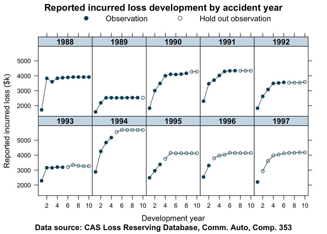
The data appears to be reasonably well behaved. Although the years converge to different levels of ultimate incurred claims, the shape of the curves look similar for most years. The accident years 1988 and 1993 show a distinctly different pattern.
Stan model
So let’s put this model into Stan. Again, I follow Glenn’s implementation, but I have changed some of the variable names and added some lines in the generated quantities block to predict incurred claims for the test data period.
library(rstan)
rstan_options(auto_write = TRUE)
options(mc.cores = parallel::detectCores())
data{
int <lower=1> len_data; // number of rows with data
int<lower=1> len_pred; // number of rows to predict
// indicator of first origin period
int<lower=0, upper=1> origin1id[len_data + len_pred];
real logprem[len_data + len_pred];
real logloss[len_data];
int<lower=1> origin[len_data + len_pred]; // origin period
int<lower=1> dev[len_data + len_pred]; // development period
}
transformed data{
int n_origin = max(origin);
int n_dev = max(dev);
int len_total = len_data + len_pred;
}
parameters{
real r_alpha[n_origin - 1];
real r_beta[n_dev - 1];
real log_elr;
real<lower=0, upper=100000> a_ig[n_dev];
real<lower=0, upper=1> r_rho;
real logloss_pred[len_pred];
}
transformed parameters{
real alpha[n_origin];
real beta[n_dev];
real sig2[n_dev];
real sig[n_dev];
real mu[len_data];
real mu_pred[len_pred];
real <lower=-1, upper=1> rho;
rho = -2*r_rho + 1;
alpha[1] = 0;
for (i in 2:n_origin){
alpha[i] = r_alpha[i-1];
}
for (i in 1:(n_dev - 1)){
beta[i] = r_beta[i];
}
beta[n_dev] = 0;
// Create ascending set of sig2
sig2[n_dev] = gamma_cdf(1/a_ig[n_dev],1,1); // map into [0,1]
for (i in 1:(n_dev-1)){
sig2[n_dev - i] = sig2[n_dev + 1 - i] + gamma_cdf(1/a_ig[i],1,1);
}
for (i in 1:n_dev){
sig[i] = sqrt(sig2[i]);
}
// first origin and dev period (top left corner of triangle)
mu[1] = logprem[1] + log_elr + beta[dev[1]];
for (i in 2:len_data){
mu[i] = logprem[i] + log_elr + alpha[origin[i]] + beta[dev[i]] +
rho*(logloss[i-1] - mu[i-1]) * origin1id[i];
}
mu_pred[1] = logprem[(len_data) + 1] + alpha[origin[len_data + 1]] +
log_elr + beta[dev[len_data + 1]] +
rho*(logloss[len_data] - mu[len_data]) * origin1id[len_data + 1];
for (i in 2:len_pred){
mu_pred[i] = logprem[len_data + i] + alpha[origin[len_data + i]] +
log_elr + beta[dev[len_data + i]] +
rho*(logloss_pred[i-1] - mu_pred[i-1]) * origin1id[len_data + i];
}
}
model {
log_elr ~ normal(0, 1);
r_alpha ~ normal(0, sqrt(10/1.0));
r_beta ~ normal(0, sqrt(10/1.0));
a_ig ~ inv_gamma(1,1); // inverse gamma for numerical resaons
r_rho ~ beta(2,2);
// model where we have data
for (i in 1:(len_data)){
logloss[i] ~ normal(mu[i], sig[dev[i]]);
}
// model where data is missing, the prediction period
for (i in 1:(len_pred)){
logloss_pred[i] ~ normal(mu_pred[i], sig[dev[len_data + i]]);
}
}
generated quantities{
vector[len_data] log_lik;
vector[len_total] ppc_loss;
for (i in 1:len_data){
log_lik[i] = normal_lpdf(logloss[i] | mu[i], sig[dev[i]]);
}
// simulate posterior predicted losses
for (i in 1:len_data){
ppc_loss[i] = exp(normal_rng(mu[i], sig[dev[i]]));
}
for (i in 1:len_pred){
ppc_loss[len_data + i] = exp(normal_rng(mu_pred[i], sig[dev[len_data + i]]));
}
}The next code block prepares the data as an input for Stan.
createStanDataList <- function(lossData){
  with(lossData, {
    train_idx <- !is.na(loss_train)
    list(
      len_data = sum(train_idx),
      len_pred = sum(!train_idx),
      logprem = log(premium),
      logloss = log(loss_train[train_idx]),
      origin = origin,
      dev = dev,
      origin1id = origin1id)
  })
}
stan_data <- createStanDataList(lossData)
Model run for company 353
Finally, we can run our Stan model for company 353.
fitCCL353 <- sampling(CCLmodel,
                      data=stan_data,
                      seed = 1234, iter = 4000,
                      control=list(adapt_delta = 0.99,
                                   max_treedepth = 10))
## Warning: There were 4824 transitions after warmup that exceeded the maximum treedepth. Increase max_treedepth above 10. See
## http://mc-stan.org/misc/warnings.html#maximum-treedepth-exceeded## Warning: There were 4 chains where the estimated Bayesian Fraction of Missing Information was low. See
## http://mc-stan.org/misc/warnings.html#bfmi-low## Warning: Examine the pairs() plot to diagnose sampling problems## Warning: Bulk Effective Samples Size (ESS) is too low, indicating posterior means and medians may be unreliable.
## Running the chains for more iterations may help. See
## http://mc-stan.org/misc/warnings.html#bulk-essStan comes back with a couple of warnings and messages to investigate the model in more detail.
I get pretty much the same output as Glenn (see slides 19, 20):
print(fitCCL353,
      pars=c("alpha", "beta", "rho", "log_elr", "sig"),
      probs=c(0.025, 0.975))
## Inference for Stan model: 478cdd2fd5b96bedcdb4ea70c25e0f67.
## 4 chains, each with iter=4000; warmup=2000; thin=1;
## post-warmup draws per chain=2000, total post-warmup draws=8000.
##
## mean se_mean sd 2.5% 97.5% n_eff Rhat
## alpha[1] 0.00 NaN 0.00 0.00 0.00 NaN NaN
## alpha[2] -0.26 0.00 0.02 -0.29 -0.23 2809 1.00
## alpha[3] 0.11 0.00 0.02 0.06 0.15 1315 1.00
## alpha[4] 0.21 0.00 0.03 0.16 0.26 1356 1.00
## alpha[5] 0.01 0.00 0.03 -0.06 0.07 752 1.00
## alpha[6] -0.06 0.00 0.04 -0.13 0.03 1695 1.00
## alpha[7] 0.45 0.00 0.06 0.33 0.56 1477 1.00
## alpha[8] 0.03 0.00 0.08 -0.13 0.20 1791 1.00
## alpha[9] 0.15 0.00 0.14 -0.14 0.43 1352 1.00
## alpha[10] 0.18 0.01 0.29 -0.36 0.77 1316 1.01
## beta[1] -0.59 0.00 0.11 -0.83 -0.38 4223 1.00
## beta[2] -0.19 0.00 0.07 -0.32 -0.05 3015 1.00
## beta[3] -0.10 0.00 0.05 -0.20 0.00 1861 1.00
## beta[4] -0.03 0.00 0.04 -0.10 0.05 1543 1.00
## beta[5] -0.01 0.00 0.03 -0.07 0.05 1180 1.00
## beta[6] 0.00 0.00 0.03 -0.06 0.06 1205 1.00
## beta[7] 0.00 0.00 0.03 -0.05 0.06 1031 1.00
## beta[8] 0.01 0.00 0.02 -0.05 0.06 1314 1.00
## beta[9] 0.00 0.00 0.02 -0.05 0.05 1662 1.00
## beta[10] 0.00 NaN 0.00 0.00 0.00 NaN NaN
## rho 0.17 0.00 0.21 -0.27 0.55 2542 1.00
## log_elr -0.39 0.00 0.01 -0.43 -0.37 1216 1.00
## sig[1] 0.26 0.00 0.09 0.14 0.51 3494 1.00
## sig[2] 0.15 0.00 0.04 0.09 0.26 3836 1.00
## sig[3] 0.09 0.00 0.03 0.05 0.16 1865 1.00
## sig[4] 0.06 0.00 0.02 0.03 0.11 547 1.01
## sig[5] 0.04 0.00 0.02 0.02 0.09 374 1.01
## sig[6] 0.04 0.00 0.02 0.02 0.07 310 1.01
## sig[7] 0.03 0.00 0.01 0.01 0.06 309 1.01
## sig[8] 0.02 0.00 0.01 0.01 0.05 295 1.01
## sig[9] 0.02 0.00 0.01 0.01 0.04 299 1.01
## sig[10] 0.01 0.00 0.01 0.00 0.03 341 1.01
##
## Samples were drawn using NUTS(diag_e) at Sun Jan 12 22:34:19 2020.
## For each parameter, n_eff is a crude measure of effective sample size,
## and Rhat is the potential scale reduction factor on split chains (at
## convergence, Rhat=1).Some of the parameters don’t appear significant, such as \(\beta_5\) to \(\beta_9\), but then again they shouldn’t have done any harm here either, as they will have had little impact.
However, I am most interested in comparing the posterior predictive distribution with the training and test data. How does the model perform out of sample?
The next code chunk extracts the 95% credible interval from the posterior predictive simulated losses and plots the output.
createPlotData <- function(stanfit, data, probs=c(0.25, 0.975)){

  ppc_loss <- as.matrix(extract(stanfit, "ppc_loss")$ppc_loss)
  ppc_loss_summary <- cbind(
    mean=apply(ppc_loss, 2, mean),
    t(apply(ppc_loss, 2, quantile, probs=probs))
  )
  colnames(ppc_loss_summary) = c(
    "Y_pred_mean",
    paste0("Y_pred_cred", gsub("\\.", "", probs[1])),
    paste0("Y_pred_cred", gsub("\\.", "", probs[2])))

  return(cbind(ppc_loss_summary, data))
}
plotDevBananas <- function(x, data, company_code,
xlab="Development year",
ylab="Reported incurred loss ($k)",
main="Correlated Log-normal Chain Ladder Model",
...){
key <- list(
rep=FALSE,
lines=list(col=c("#00526D", "#00526D", "purple"),
type=c("p", "p", "l"),
pch=c(19, 1, NA)),
text=list(lab=c("Observation", "Hold out observation", "Mean estimate")),
rectangles = list(col=adjustcolor("yellow", alpha.f=0.5), border="grey"),
text=list(lab="95% Posterior prediction interval"))
xyplot(x, data=data,as.table=TRUE,xlab=xlab, ylab=ylab, main=main,
sub=paste("Data source: CAS Loss Reserving Database,",
"Comm. Auto, Comp.",
company_code),
scales=list(alternating=1), layout=c(5,2), key=key,
par.settings = list(strip.background=list(col="#CBDDE6")),
par.strip.text = list(font = 2),
panel=function(x, y){
n <- length(x)
divisor <- 5
cn <- c(1:(n/divisor))
upper <- y[cn+n/divisor*0]
lower <- y[cn+n/divisor*1]
x <- x[cn]
panel.polygon(c(x, rev(x)), c(upper, rev(lower)),
col = adjustcolor("yellow", alpha.f = 0.5),
border = "grey")
panel.lines(x, y[cn+n/divisor*2], col="purple")
panel.points(x, y[cn+n/divisor*4], lwd=1, col="#00526D")
panel.points(x, y[cn+n/divisor*3], lwd=1, pch=19, col="#00526D")
}, ...)
}plotData <- createPlotData(fitCCL353, data=lossData)
plotDevBananas(Y_pred_cred025 + Y_pred_cred0975 + Y_pred_mean +
loss_train + loss_test ~ dev | factor(accident_year),
data=plotData, company_code = 353)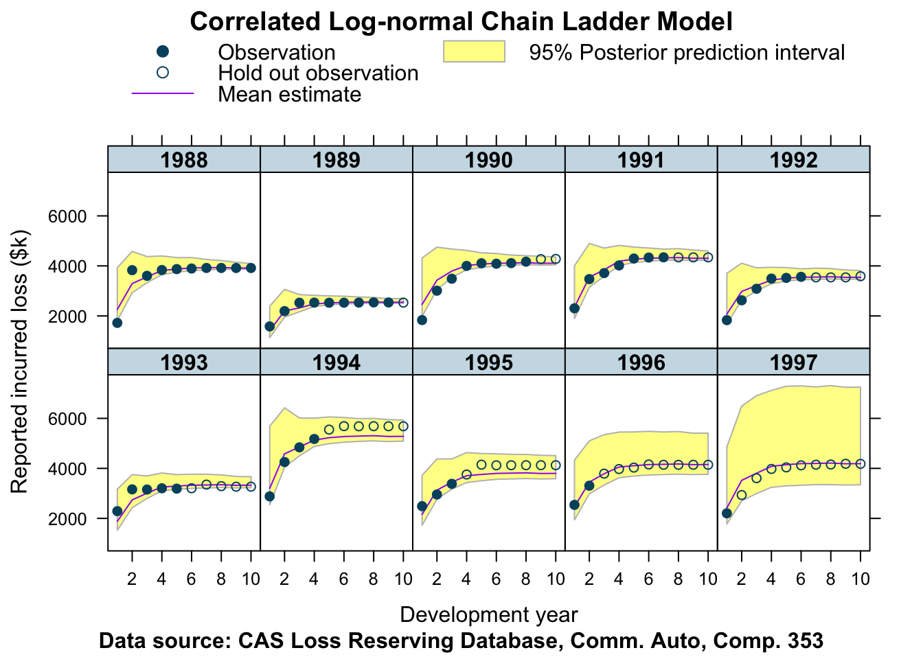
This looks pretty good!
We can see for the older years that the credible interval shrinks as the development years progress. The skewness of the log-normal distribution is clearly visible for the most recent accident years. In all cases the hold out observations are within the 95% posterior prediction interval, often very close to the mean, apart from the years 1994 and 1995, where we observe a more unusual pattern in the data.
Finally, here is the distribution of the ‘population’ loss ratio \(\ell\) across all accident years and correlation parameter \(\rho\).
summary(elr <- exp(extract(fitCCL353, "log_elr")$log_elr))## Min. 1st Qu. Median Mean 3rd Qu. Max.
## 0.6033 0.6695 0.6740 0.6739 0.6786 0.7380summary(rho <- extract(fitCCL353, "rho")$rho)## Min. 1st Qu. Median Mean 3rd Qu. Max.
## -0.86328 0.03551 0.18278 0.17077 0.31764 0.87749The distribution of \(\rho\) is very interesting. Many of the traditional reserving methods, including the Mack-chain-ladder model assume that the accident years are independent. However, for this data set it is unlikely to be valid. Indeed, the probability of a positive correlation is 80%.
library(MASS); library(latex2exp)
truehist(rho, col="skyblue", xlab=TeX("$\\\\rho$"));
abline(v=0, col=2)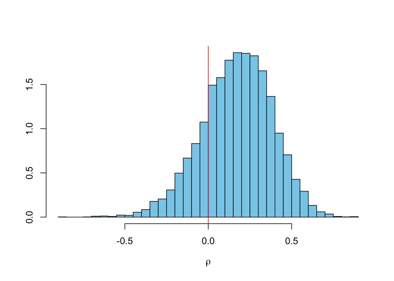
Company 833
Let’s look at another company. Here is the data for company 833.
lossData <- createLossData(CASdata, company_code = 833, loss_type="incurred")
devPlot(loss_train + loss_test
        ~ dev | factor(accident_year),
        data=lossData, company_code = 833)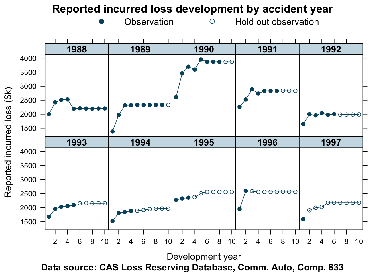
This data is not as well behaved as for company 353. The shape of the curves do vary quite a bit from one accident year to the next. Let’s find out how well our model predicts the hold out sample in this case.
stan_data <- createStanDataList(lossData)fitCCL833 <- sampling(CCLmodel,
data=stan_data,
seed = 1234, iter = 4000,
control=list(adapt_delta = 0.99,
max_treedepth = 10))## Warning: There were 28 divergent transitions after warmup. Increasing adapt_delta above 0.99 may help. See
## http://mc-stan.org/misc/warnings.html#divergent-transitions-after-warmup## Warning: There were 1443 transitions after warmup that exceeded the maximum treedepth. Increase max_treedepth above 10. See
## http://mc-stan.org/misc/warnings.html#maximum-treedepth-exceeded## Warning: There were 4 chains where the estimated Bayesian Fraction of Missing Information was low. See
## http://mc-stan.org/misc/warnings.html#bfmi-low## Warning: Examine the pairs() plot to diagnose sampling problems## Warning: Bulk Effective Samples Size (ESS) is too low, indicating posterior means and medians may be unreliable.
## Running the chains for more iterations may help. See
## http://mc-stan.org/misc/warnings.html#bulk-essStan gives messages back, which I shall ignore for the time being and instead look at my ‘banana’ plot again.
plotData <- createPlotData(fitCCL833, lossData)
plotDevBananas(Y_pred_cred025 + Y_pred_cred0975 + Y_pred_mean +
                 loss_train + loss_test ~ dev | factor(accident_year),
               data=plotData, company_code = 833)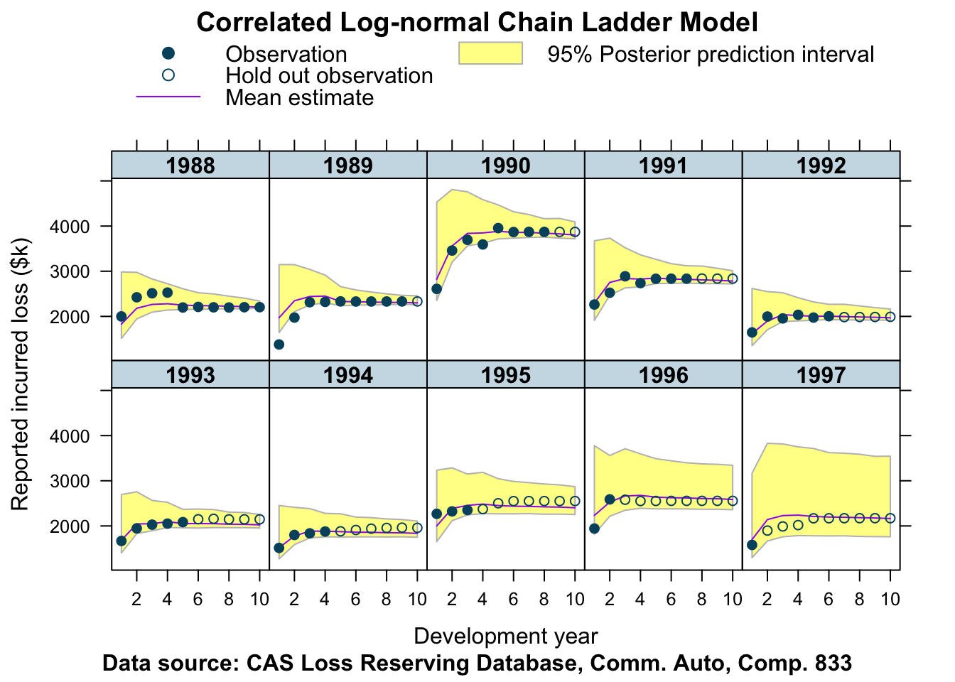
Interesting! Not too bad either.
Company 25275
Here is another company, whose data show some unusual patterns.
## Other companies
lossData <- createLossData(CASdata, company_code = 25275, loss_type="incurred")
devPlot(loss_train + loss_test
        ~ dev | factor(accident_year),
        data=lossData, company_code = 25275)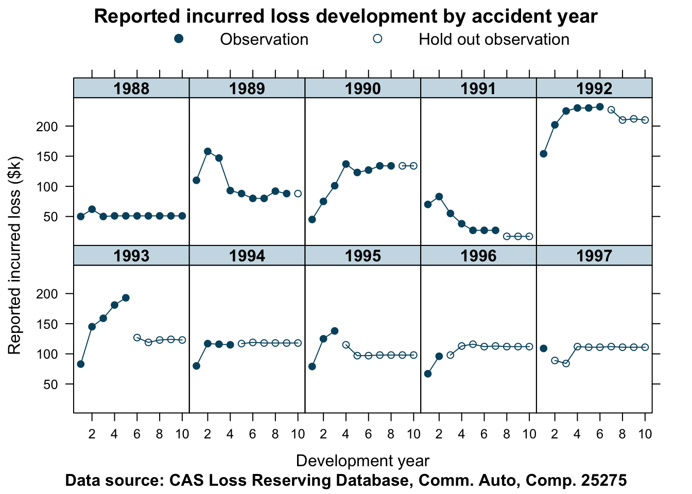
Let’s fit this data with the same model as well.
stan_data <- createStanDataList(lossData)fitCCL25275 <- sampling(CCLmodel,
data=stan_data,
seed = 1234, iter = 4000,
control=list(adapt_delta = 0.99,
max_treedepth = 10))## Warning: There were 132 divergent transitions after warmup. Increasing adapt_delta above 0.99 may help. See
## http://mc-stan.org/misc/warnings.html#divergent-transitions-after-warmup## Warning: There were 1738 transitions after warmup that exceeded the maximum treedepth. Increase max_treedepth above 10. See
## http://mc-stan.org/misc/warnings.html#maximum-treedepth-exceeded## Warning: There were 4 chains where the estimated Bayesian Fraction of Missing Information was low. See
## http://mc-stan.org/misc/warnings.html#bfmi-low## Warning: Examine the pairs() plot to diagnose sampling problems## Warning: Bulk Effective Samples Size (ESS) is too low, indicating posterior means and medians may be unreliable.
## Running the chains for more iterations may help. See
## http://mc-stan.org/misc/warnings.html#bulk-essplotData <- createPlotData(fitCCL25275, lossData)
plotDevBananas(Y_pred_cred025 + Y_pred_cred0975 + Y_pred_mean +
loss_train + loss_test ~ dev | factor(accident_year),
data=plotData, company_code = 25275,
ylim=c(0, 500))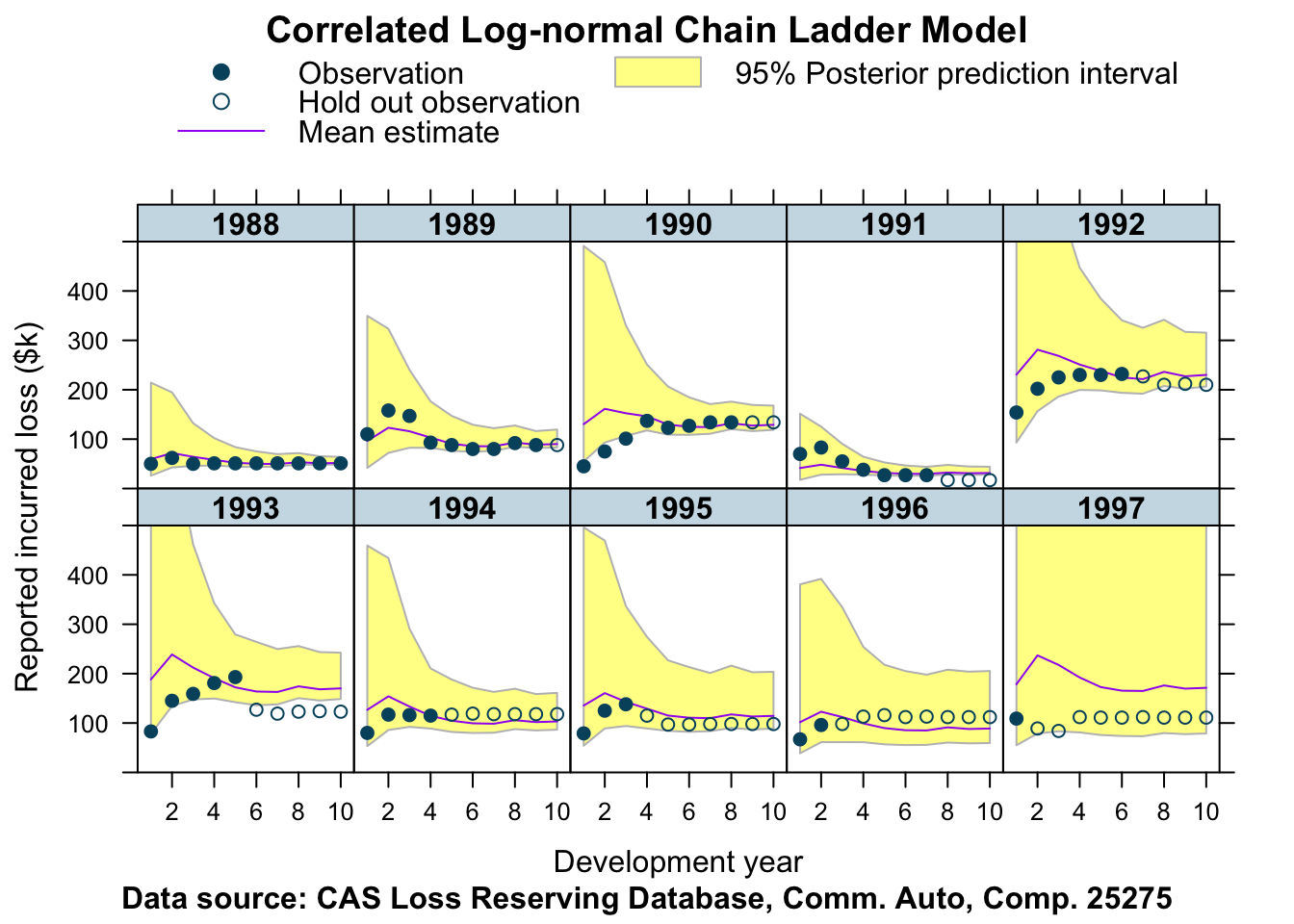
Well, what do you think about that?
References
Stochastic Loss Reserving Using Bayesian McMc Models. Glenn Meyers. CAS monograph series. Number 1. Casualty Actuarial Society. 2015
Session Info
sessionInfo()## R version 3.6.2 (2019-12-12)
## Platform: x86_64-apple-darwin15.6.0 (64-bit)
## Running under: macOS Catalina 10.15.2
##
## Matrix products: default
## BLAS: /Library/Frameworks/R.framework/Versions/3.6/Resources/lib/libRblas.0.dylib
## LAPACK: /Library/Frameworks/R.framework/Versions/3.6/Resources/lib/libRlapack.dylib
##
## locale:
## [1] en_GB.UTF-8/en_GB.UTF-8/en_GB.UTF-8/C/en_GB.UTF-8/en_GB.UTF-8
##
## attached base packages:
## [1] stats graphics grDevices utils datasets methods base
##
## other attached packages:
## [1] latex2exp_0.4.0 MASS_7.3-51.5 rstan_2.19.2 ggplot2_3.2.1
## [5] StanHeaders_2.19.0 lattice_0.20-38 data.table_1.12.8
##
## loaded via a namespace (and not attached):
## [1] Rcpp_1.0.3 compiler_3.6.2 pillar_1.4.3 prettyunits_1.1.0
## [5] tools_3.6.2 pkgbuild_1.0.6 digest_0.6.23 evaluate_0.14
## [9] lifecycle_0.1.0 tibble_2.1.3 gtable_0.3.0 pkgconfig_2.0.3
## [13] rlang_0.4.2 cli_2.0.1 parallel_3.6.2 yaml_2.2.0
## [17] blogdown_0.17 xfun_0.11 loo_2.2.0 gridExtra_2.3
## [21] withr_2.1.2 stringr_1.4.0 dplyr_0.8.3 knitr_1.26
## [25] stats4_3.6.2 grid_3.6.2 tidyselect_0.2.5 glue_1.3.1
## [29] inline_0.3.15 R6_2.4.1 processx_3.4.1 fansi_0.4.1
## [33] rmarkdown_2.0 bookdown_0.17 callr_3.4.0 purrr_0.3.3
## [37] magrittr_1.5 codetools_0.2-16 matrixStats_0.55.0 ps_1.3.0
## [41] scales_1.1.0 htmltools_0.4.0 assertthat_0.2.1 colorspace_1.4-1
## [45] stringi_1.4.5 lazyeval_0.2.2 munsell_0.5.0 crayon_1.3.4Citation
For attribution, please cite this work as:Markus Gesmann (Dec 02, 2017) Correlated log-normal chain-ladder model. Retrieved from https://magesblog.com/post/correlated-lognormal-chain-ladder-model/
@misc{ 2017-correlated-log-normal-chain-ladder-model,
author = { Markus Gesmann },
title = { Correlated log-normal chain-ladder model },
url = { https://magesblog.com/post/correlated-lognormal-chain-ladder-model/ },
year = { 2017 }
updated = { Dec 02, 2017 }
}