Changing settlement rate model for paid losses
Last week I wrote about Glenn Meyers’ correlated log-normal chain-ladder model (CCL), which he presented at the 10th Bayesian Mixer Meetup. Today, I will continue with a variant Glenn also discussed: The changing settlement log-normal chain-ladder model (CSR).
Glenn used the correlated log-normal chain-ladder model on reported incurred claims data to predict future developments.
However, when looking at paid claims data, Glenn suggested to change the model slightly. Instead allowing for correlation across accident years, he allows for a gradual shift in the payout pattern to account for a change in the claim settlement rate across accident years.
The changing settlement rate log-normal chain-ladder model
The changing settlement rate log-normal chain-ladder model looks very similar to the correlated log-normal chain-ladder model, but instead of a correlation parameter \(\rho\), we have the settlement rate \(\gamma\).
\[ \begin{align} C_{i,j} & \sim \log\mathcal{N}(\mu_{i,j}, \sigma^2_j)\\ L_i & = P_i \cdot \ell\\ \mu_{1,j} & = \log(L_1) + \beta_j \\ \mu_{i,j} & = \log(L_i) + \alpha_i + \beta_j \cdot \left(1 - \gamma\right)^{i-1} \\ & \mbox{for } i = 2, \dots, M \mbox{ and } j = 1, \dots, N+1-i \\ & \mbox{and } \alpha_1 := 0,\, \beta_N := 0\\ \sigma^2_j & = \sum_{k=j}^N a_k \\ & \mbox{with priors}\\ \alpha_i & \sim \mathcal{N}(0, 10) \\ \beta_i & \sim \mathcal{N}(0, 10) \\ \log(\ell) & \sim \mathcal{N}(0, 1) \\ \gamma & \sim \mathcal{N}(0, 0.05)\\ a_k & \sim \mbox{Uniform}(0,1)\\ &\mbox{and}\\ C_{i,j} &:=\mbox{cumulative paid claims of origin } i\mbox{, development }j \\ P_{i} & := \mbox{premium of origin } i\\ \ell & := \mbox{'population' loss ratio across all origin periods}\\ L_i & := \mbox{initial expected ultimate loss for origin } i\\ M & := \mbox{number of origin periods} \\ N & := \mbox{number of development periods} \end{align} \] A positive \(\gamma\) moves the development period component closer to zero with each origin period (accident year). Hence a speed-up of claim settlement, e.g. claims are reported and settled faster today due to technology. If \(\gamma\) is negative, the claim settlement slows down.
Let’s take a look at the paid claims data for Commercial Auto of company 353, using the R function from the previous post.
library(data.table)
CASdata <- fread("http://www.casact.org/research/reserve_data/comauto_pos.csv")
lossData <- createLossData(CASdata, company_code = 353, loss_type="paid")
devPlot(loss_train + loss_test
~ dev | factor(accident_year),
main="Paid loss development by accident year",
ylab = "Paid loss ($k)",
data=lossData, company_code = 353)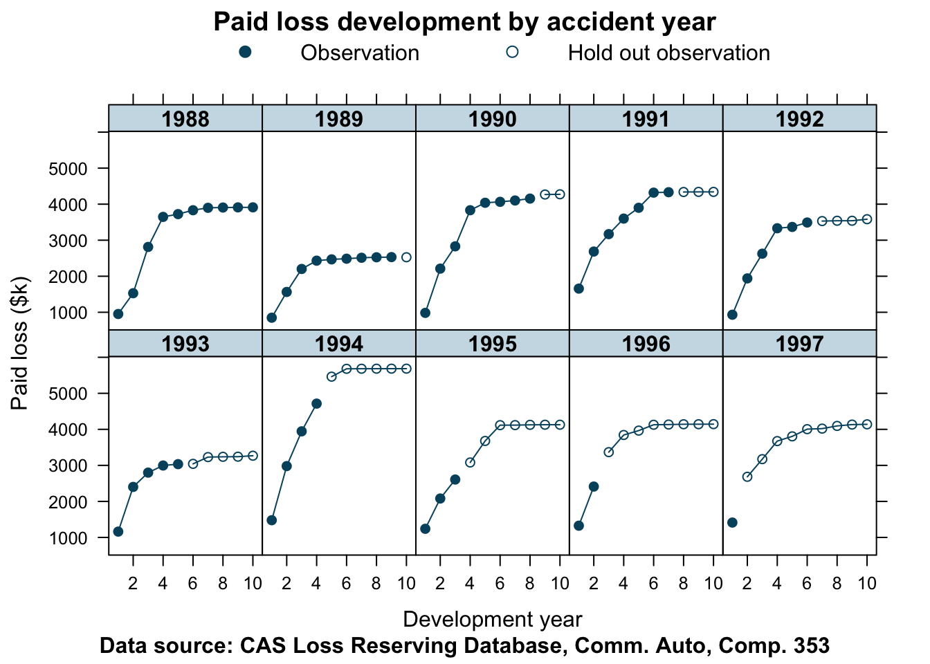
Stan model
My Stan model follows Glenn’s implementation, yet I changed some of the variable names and added lines in the generated quantities block to predict future paid claims for the test data period.
data{
  int <lower=1> len_data; // number of rows with data
  int<lower=1> len_pred; // number of rows to predict
  real logprem[len_data + len_pred];
  real logloss[len_data];
  int<lower=1> origin[len_data + len_pred]; // origin period
  int<lower=1> dev[len_data + len_pred]; // development period
}
transformed data{
  int n_origin = max(origin);
  int n_dev = max(dev);
  int len_total = len_data + len_pred;
}
parameters{
  real r_alpha[n_origin - 1];
  real r_beta[n_dev - 1];
  real log_elr;
  real<lower=0, upper=100000> a_ig[n_dev];
  real gamma;
  real logloss_pred[len_pred];
}
transformed parameters{
  real alpha[n_origin];
  real beta[n_dev];
  real speedup[n_origin];
  real sig2[n_dev];
  real sig[n_dev];
  real mu[len_data];
  real mu_pred[len_pred];

  alpha[1] = 0;
  for (i in 2:n_origin){
    alpha[i] = r_alpha[i-1];
  }
  for (i in 1:(n_dev - 1)){
    beta[i] = r_beta[i];
  }
  beta[n_dev] = 0;

  speedup[1] = 1;
  for (i in 2:n_origin){
    speedup[i] = speedup[i-1]*(1 - gamma);
  }
  // Create ascending set of sig2
  sig2[n_dev] = gamma_cdf(1/a_ig[n_dev],1,1); // map into [0,1]
  for (i in 1:(n_dev-1)){
    sig2[n_dev - i] = sig2[n_dev + 1 - i] + gamma_cdf(1/a_ig[i],1,1);
  }
  for (i in 1:n_dev){
    sig[i] = sqrt(sig2[i]);
  }
  for (i in 1:len_data){
    mu[i] = logprem[i] + log_elr + alpha[origin[i]] +
                        beta[dev[i]] * speedup[origin[i]];
  }
  for (i in 1:len_pred){
    mu_pred[i] = logprem[len_data + i] + log_elr + alpha[origin[len_data + i]] +
                        beta[dev[len_data + i]] * speedup[origin[len_data + i]];
  }
}
model {
  log_elr ~ normal(0, 1);
  r_alpha ~ normal(0, sqrt(10/1.0));
  r_beta ~ normal(0, sqrt(10/1.0));
  a_ig ~ inv_gamma(1,1); // inverse gamma for numerical resaons
  gamma ~ normal(0,0.05);
  // model where we have data
  for (i in 1:(len_data)){
    logloss[i] ~ normal(mu[i], sig[dev[i]]);
  }
  // model where data is missing, the prediction period
  for (i in 1:(len_pred)){
    logloss_pred[i] ~ normal(mu_pred[i], sig[dev[len_data + i]]);
  }
}
generated quantities{
  vector[len_data] log_lik;
  vector[len_total] ppc_loss;

  for (i in 1:len_data){
    log_lik[i] = normal_lpdf(logloss[i] | mu[i], sig[dev[i]]);
  }
  // simulate posterior predicted losses
  for (i in 1:len_data){
    ppc_loss[i] = exp(normal_rng(mu[i], sig[dev[i]]));
  }
  for (i in 1:len_pred){
    ppc_loss[len_data + i] = exp(normal_rng(mu_pred[i], sig[dev[len_data + i]]));
  }
}
Model run for company 353
Let’s run this Stan model for company 353.
stan_data <- createStanDataList(lossData)
fitCSR353 <- sampling(CSRmodel,
                      data=stan_data,
                      seed = 1234, iter = 4000,
                      control=list(adapt_delta = 0.99,
                                   max_treedepth = 10))
## Warning: There were 3908 transitions after warmup that exceeded the maximum treedepth. Increase max_treedepth above 10. See
## http://mc-stan.org/misc/warnings.html#maximum-treedepth-exceeded## Warning: There were 4 chains where the estimated Bayesian Fraction of Missing Information was low. See
## http://mc-stan.org/misc/warnings.html#bfmi-low## Warning: Examine the pairs() plot to diagnose sampling problems## Warning: Bulk Effective Samples Size (ESS) is too low, indicating posterior means and medians may be unreliable.
## Running the chains for more iterations may help. See
## http://mc-stan.org/misc/warnings.html#bulk-essJust like last week I review the model in my ‘banana’ chart.
plotData <- createPlotData(fitCSR353, data=lossData)
plotDevBananas(Y_pred_cred025 + Y_pred_cred0975 +
                 Y_pred_mean + loss_train +
                 loss_test ~ dev | factor(accident_year),
               data=plotData, company_code = 353,
               ylab="Paid loss ($k)",
               main="Changing Settlement Rate Chain Ladder Model")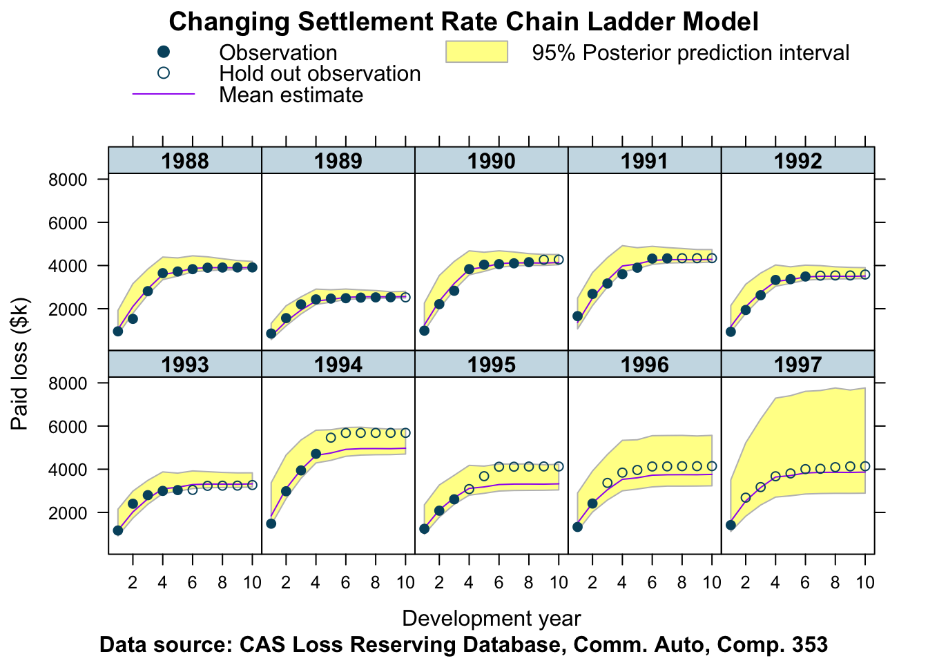
This output looks reasonable, but not as good as the output of the correlated log-normal chain-ladder model. The accident years of 1994 - 1997 have been under-predicted.
Let’s take a look at the variable \(\gamma\).
out353 <- extract(fitCSR353)
library(MASS); library(latex2exp)
truehist(out353$gamma, col="skyblue", xlab=TeX("$\\\\gamma$"));
abline(v=mean(out353$gamma), col="blue", lwd=2)
abline(v=0, col=2)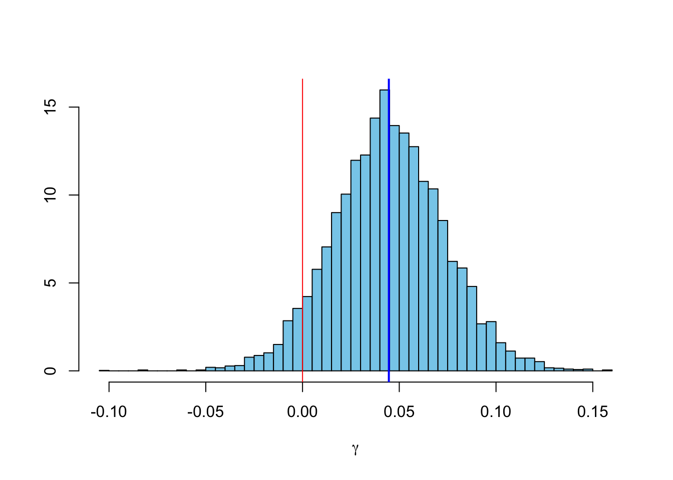
With a mean \(\gamma\) of 4.5% we expect a speed-up in the claims settlement pattern from one accident year to the next. Given that \(\exp{\left(\beta_j \cdot (1-\gamma)^{(i-1)}\right)}\) describes the paid to ultimate development we can plot the development curves for the different origin years.
M <- max(stan_data$origin)
beta <- apply(out353$beta, 2, mean)
gamma <- mean(out353$gamma)
Beta <- matrix(rep(beta, M), nrow=M, byrow = TRUE)
BetaOrigin <- exp(sweep(Beta, 1, (1 - gamma)^(1:M-1), "*"))
library(ChainLadder)
BetaOriginLong <- as.data.frame(as.triangle(BetaOrigin))
library(latticeExtra)
xyplot(value*100 ~ dev, groups=as.numeric(origin),
data=BetaOriginLong, t="b",
main="Claims settlement patterns by origin year",
xlab="Development year",
ylab="Claims paid to ultimate (%)",
auto.key = list(space="right", title="Origin", cex=0.75),
par.settings = theEconomist.theme(box = "grey"))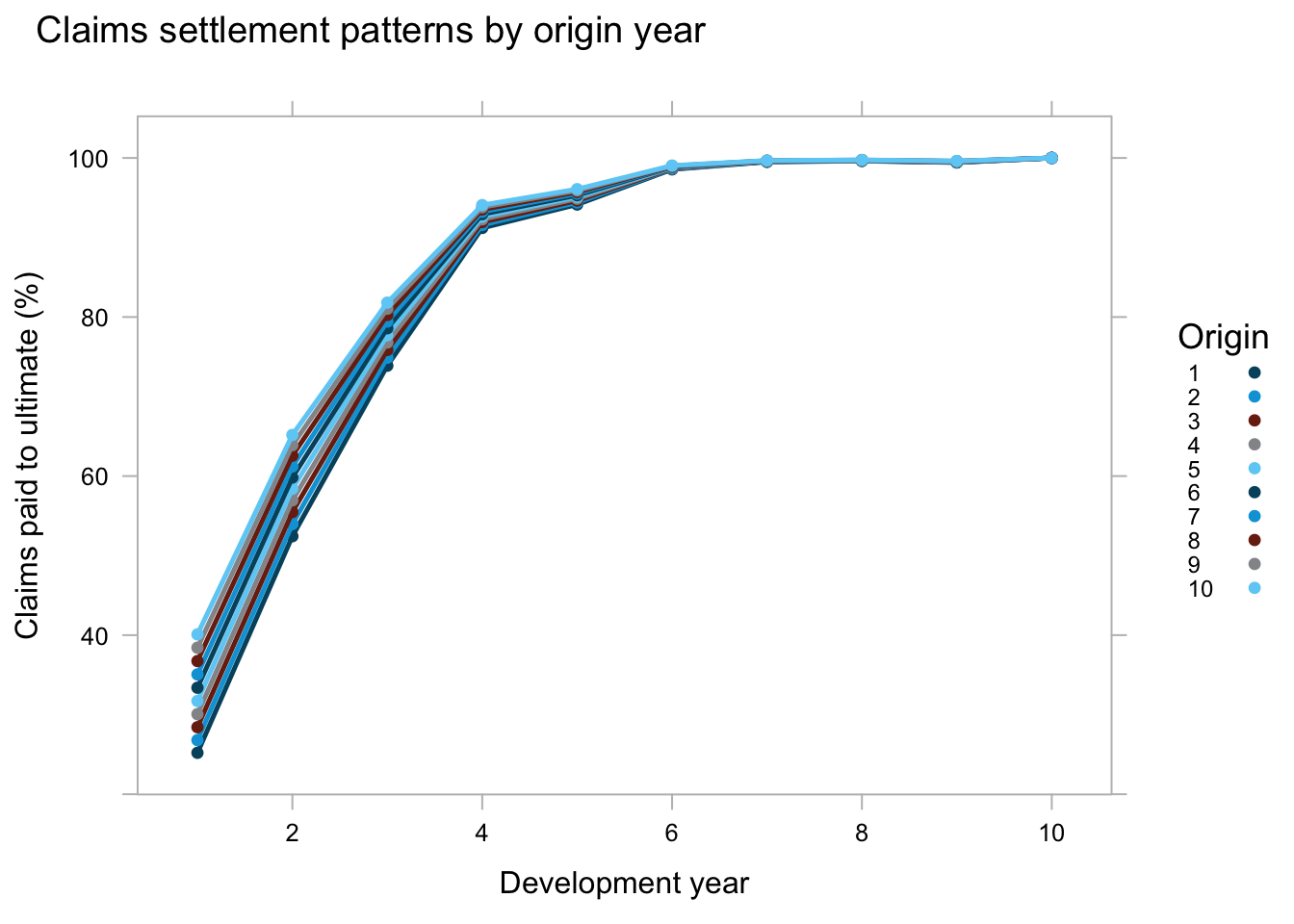 The chart describes nicely how we expect the younger accident years to develop faster than older years.
In a similar way we can look at \(\,\ell \cdot \exp{\alpha_i}\), which describes how the ultimate loss ratio varies from the expected loss ratio across accident years.
mean_ulr <- apply(exp(
  sweep(out353$alpha, 1, out353$log_elr, "+")), 2, mean)
cred_ulr <- t(apply(exp(
  sweep(out353$alpha, 1, out353$log_elr, "+")), 2,
  quantile, c(0.0275, 0.975)))
current_ilr <- lossData[cal==10, loss/premium]
latest_ilr <- lossData[dev==10, loss/premium]
ay <- unique(lossData$accident_year)
DT <- data.table(ay, `mean ulr`=mean_ulr*100,
                 `lwr cred ulr`=cred_ulr[,1]*100,
                 `upr cred ulr`=cred_ulr[,2]*100,
                 `latest ilr`=latest_ilr*100,
                 `current ilr`=current_ilr*100)
plotDevBananas(`lwr cred ulr` + `upr cred ulr` +
                 `mean ulr` + `current ilr` +
                 `latest ilr` ~ ay,
               data=DT, company_code = 353,
               ylab="Loss ratio (%)", xlab="Accident year",
               main="Changing Settlement Rate Chain Ladder Model",
               layout=c(1,1))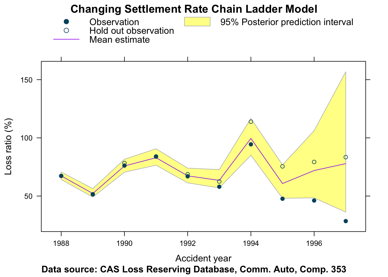
For this data set it appears that although the CSR model recognised the speed-up in claim settlements, the CCL model with reported incurred claims provided the better fit. Indeed, perhaps the speed-up in the settlement rate is reversed in the younger years?
Company 833
Let’s test the model again for two other companies. Again I start with company 833.
lossData <- createLossData(CASdata, company_code = 833, loss_type="paid")
stan_data <- createStanDataList(lossData)
fitCSR833 <- sampling(CSRmodel,
data=stan_data,
seed = 1234, iter = 4000,
control=list(adapt_delta = 0.99,
max_treedepth = 10))## Warning: There were 2649 transitions after warmup that exceeded the maximum treedepth. Increase max_treedepth above 10. See
## http://mc-stan.org/misc/warnings.html#maximum-treedepth-exceeded## Warning: There were 4 chains where the estimated Bayesian Fraction of Missing Information was low. See
## http://mc-stan.org/misc/warnings.html#bfmi-low## Warning: Examine the pairs() plot to diagnose sampling problems## Warning: Bulk Effective Samples Size (ESS) is too low, indicating posterior means and medians may be unreliable.
## Running the chains for more iterations may help. See
## http://mc-stan.org/misc/warnings.html#bulk-essplotData <- createPlotData(fitCSR833, lossData)
plotDevBananas(Y_pred_cred025 + Y_pred_cred0975 + Y_pred_mean +
loss_train + loss_test ~ dev | factor(accident_year),
data=plotData, company_code = 833,
ylab="Paid loss ($k)",
main="Changing Settlement Rate Chain Ladder Model")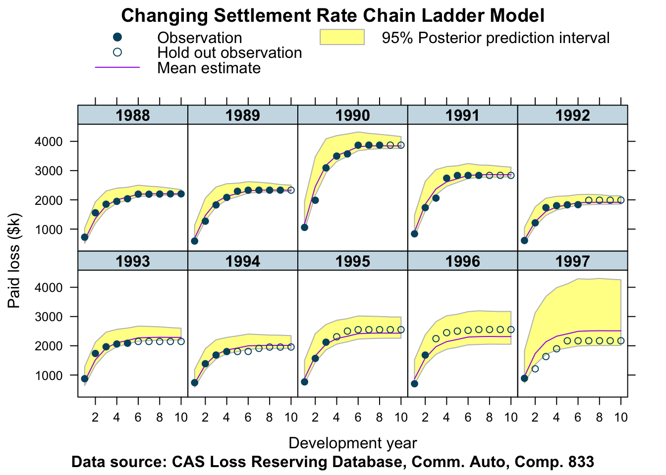
Again, the output looks reasonable, but the predictions for the most recent accident years are not as good as with the correlated log-normal chain-ladder model.
Company 25275
lossData <- createLossData(CASdata, company_code = 25275, loss_type="paid")
stan_data <- createStanDataList(lossData)
fitCSR25275 <- sampling(CSRmodel,
data=stan_data,
seed = 1234, iter = 4000,
control=list(adapt_delta = 0.99,
max_treedepth = 10))## Warning: There were 30 divergent transitions after warmup. Increasing adapt_delta above 0.99 may help. See
## http://mc-stan.org/misc/warnings.html#divergent-transitions-after-warmup## Warning: There were 190 transitions after warmup that exceeded the maximum treedepth. Increase max_treedepth above 10. See
## http://mc-stan.org/misc/warnings.html#maximum-treedepth-exceeded## Warning: There were 1 chains where the estimated Bayesian Fraction of Missing Information was low. See
## http://mc-stan.org/misc/warnings.html#bfmi-low## Warning: Examine the pairs() plot to diagnose sampling problemsplotData <- createPlotData(fitCSR25275, lossData)
plotDevBananas(Y_pred_cred025 + Y_pred_cred0975 + Y_pred_mean +
loss_train + loss_test ~ dev | factor(accident_year),
data=plotData, company_code = 25275,
ylim=c(0, 500),
ylab="Paid loss ($k)",
main="Changing Settlement Rate Chain Ladder Model")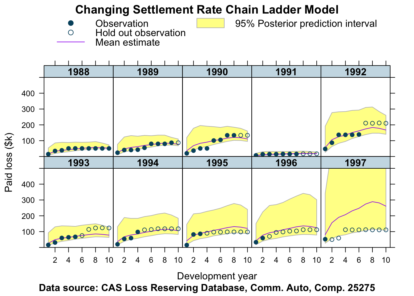
Given the data of company 25275 I am surprised how will the model works, perhaps even better than last week’s model.
References
Stochastic Loss Reserving Using Bayesian McMc Models. Glenn Meyers. CAS monograph series. Number 1. Casualty Actuarial Society. 2015
Session Info
sessionInfo()## R version 3.6.2 (2019-12-12)
## Platform: x86_64-apple-darwin15.6.0 (64-bit)
## Running under: macOS Catalina 10.15.2
##
## Matrix products: default
## BLAS: /Library/Frameworks/R.framework/Versions/3.6/Resources/lib/libRblas.0.dylib
## LAPACK: /Library/Frameworks/R.framework/Versions/3.6/Resources/lib/libRlapack.dylib
##
## locale:
## [1] en_GB.UTF-8/en_GB.UTF-8/en_GB.UTF-8/C/en_GB.UTF-8/en_GB.UTF-8
##
## attached base packages:
## [1] stats graphics grDevices utils datasets methods base
##
## other attached packages:
## [1] latticeExtra_0.6-29 ChainLadder_0.2.10 latex2exp_0.4.0
## [4] MASS_7.3-51.5 rstan_2.19.2 ggplot2_3.2.1
## [7] StanHeaders_2.19.0 lattice_0.20-38 data.table_1.12.8
##
## loaded via a namespace (and not attached):
## [1] nlme_3.1-143 matrixStats_0.55.0 RColorBrewer_1.1-2 tools_3.6.2
## [5] backports_1.1.5 R6_2.4.1 lazyeval_0.2.2 colorspace_1.4-1
## [9] systemfit_1.1-24 withr_2.1.2 tidyselect_0.2.5 gridExtra_2.3
## [13] prettyunits_1.1.0 processx_3.4.1 curl_4.3 compiler_3.6.2
## [17] cli_2.0.1 biglm_0.9-1 sandwich_2.5-1 bookdown_0.17
## [21] scales_1.1.0 lmtest_0.9-37 callr_3.4.0 stringr_1.4.0
## [25] digest_0.6.23 foreign_0.8-74 minqa_1.2.4 rmarkdown_2.0
## [29] rio_0.5.16 jpeg_0.1-8.1 pkgconfig_2.0.3 htmltools_0.4.0
## [33] rlang_0.4.2 readxl_1.3.1 zoo_1.8-7 dplyr_0.8.3
## [37] zip_2.0.4 car_3.0-6 inline_0.3.15 magrittr_1.5
## [41] loo_2.2.0 Matrix_1.2-18 Rcpp_1.0.3 munsell_0.5.0
## [45] fansi_0.4.1 abind_1.4-5 actuar_2.3-3 lifecycle_0.1.0
## [49] stringi_1.4.5 yaml_2.2.0 carData_3.0-3 expint_0.1-6
## [53] pkgbuild_1.0.6 plyr_1.8.5 grid_3.6.2 parallel_3.6.2
## [57] forcats_0.4.0 crayon_1.3.4 haven_2.2.0 splines_3.6.2
## [61] hms_0.5.3 zeallot_0.1.0 knitr_1.26 ps_1.3.0
## [65] pillar_1.4.3 reshape2_1.4.3 codetools_0.2-16 stats4_3.6.2
## [69] glue_1.3.1 evaluate_0.14 blogdown_0.17 png_0.1-7
## [73] vctrs_0.2.1 cellranger_1.1.0 gtable_0.3.0 purrr_0.3.3
## [77] assertthat_0.2.1 xfun_0.11 openxlsx_4.1.4 tweedie_2.3.2
## [81] coda_0.19-3 tibble_2.1.3 statmod_1.4.33 cplm_0.7-8Citation
For attribution, please cite this work as:Markus Gesmann (Dec 10, 2017) Changing settlement rate model for paid losses. Retrieved from https://magesblog.com/post/changing-settlement-rate-model-for-paid-losses/
@misc{ 2017-changing-settlement-rate-model-for-paid-losses,
author = { Markus Gesmann },
title = { Changing settlement rate model for paid losses },
url = { https://magesblog.com/post/changing-settlement-rate-model-for-paid-losses/ },
year = { 2017 }
updated = { Dec 10, 2017 }
}