Portfolio Allocation for Bayesian Dummies
This post is about the Black-Litterman (BL) model for asset allocation and the basis of my talk at the Dublin Data Science Meet-up. The original BL paper (Black and Litterman (1991)) is over 30 years old and builds on the ideas of modern portfolio theory by Harry Markowitz (Markowitz (1952)). A good introduction to the BL model is (Idzorek (2005)) or (Maggiar (2009)).
I am not sure how much the model is used by investment professionals, as many of the underlying assumptions may not hold true in the real world. However, the model uses some great ideas, including Bayes’ rule, to combine different pieces of information to form a more robust view that are worth exploring and are probably applicable in other fields. For the avoidance of doubt this post should not be regarded as financial advice.
Motivation
What’s the problem the BL model is addressing?
According to modern portfolio theory (MPT) investors are trying to derive assets weights for their portfolio such that the returns are maximised while the risk is minimised. MPT is also often called mean-variance analysis, as the ‘optimal’ portfolio weights (\(w^*\)) can be found using the mean returns (\(\mu\)), covariance matrix (\(\Sigma\)) and investor’s risk aversion coefficient (\(\lambda\)):
\[ \begin{aligned} w^* & = \frac{1}{\lambda} \Sigma^{-1} \mu \\ \end{aligned} \]
Although Markowitz developed a theoretically solid framework, it is prone to large estimation errors when used with sample moments for the mean and variance. The BL model starts with an asset allocation based on the equilibrium assumption (based on market capitalisation) and then modifies this allocation by considering the opinions of the investor regarding future asset performance, including uncertainties.
The neat idea of the BL model is how it uses Bayesian updating to weight and map experts’ views to market data. Some of the concepts are very similar to the Kalman filter.
I will walk through the ideas in several steps:
- Bayesian updating
- Defining prior, observations and the Kalman trick
- Example application of the BL model
Bayesian updating
The starting point is that we assume the returns of our assets follow a multivariate normal distribution, i.e., for \(k\) assets the returns can be described as:
\[ \begin{aligned} r|(\mu, \Sigma) & \sim \mathsf{Normal}(\mu, \Sigma)\\ \end{aligned} \]
That’s the likelihood distribution explaining how we believe the data is generated with known parameters.
Let’s assume the covariance matrix \(\Sigma\) is known, but that we are uncertain about the mean return \(\mu\).
Suppose experts have provided us with a prior guess on \(\mu\), which we name \(\mu_0\), and their degree of certainty, as expressed by the covariance \(\Sigma_0\). The ‘real’ \(\mu\) is believed to follow a multivariate normal distribution with parameters \(\mu_0\) and \(\Sigma_0:\)
\[ \begin{aligned} \mu & \sim \mathsf{Normal}\left(\mu_0, \Sigma_0\right)\\ \end{aligned} \]
That’s the prior parameter distribution.
In addition, suppose we have collected return data \(r_D\) that we believe came from our above likelihood distribution.
Bayes rules tells us how we can use the likelihood and prior distribution to update our belief about the parameters \(\theta\), after we have observed the data \(D\):
\[ \begin{aligned} P(\theta | D) & = \frac{P(D|\theta) P(\theta)}{P(D)}\\ \end{aligned} \]
In our case using the multivariate normal distributions with known covariances the updated posterior hyper-parameters can be calculated as (see conjugate prior):
\[ \begin{aligned} \mu_1 & = \left(\Sigma_0^{-1} + n \Sigma^{-1}\right)^{-1} \left(\Sigma_0^{-1}\mu_0 + n \Sigma^{-1} \bar{r}\right) \\ \Sigma_1 & = \left(\Sigma_0^{-1} + n \Sigma^{-1}\right)^{-1} \end{aligned} \]
Here \(\bar{r}\) is the sample average of \(r_D\) over the data.
The updated hyper-parameters \(\mu_1, \Sigma_1\) are basically credibility weighted averages.
Using the matrix inversion identity:
\[ \begin{aligned} (A^{-1} + B^{-1})^{-1} & = A - A (A + B)^{-1}A = A (A + B)^{-1} B \end{aligned} \]
the above expression can also be written as
\[ \begin{aligned} \mu_1 & = \mu_0 + \Sigma_0 \left(\Sigma_0 + n \Sigma\right)^{-1} \left( \bar{r} - \mu_0\right) \\ \Sigma_1 & = \Sigma_0 - \Sigma_0 \left(\Sigma_0 + n \Sigma\right)^{-1}\Sigma_0 \end{aligned} \]
The posterior predictive distribution, i.e., generating ‘new’ data \(\tilde{r}\), given the observations thus far, then uses the updated posterior mean \(\mu_1\) and covariance \(\Sigma_1\), plus the known uncertainty \(\Sigma\) from the likelihood:
\[ \begin{aligned} \tilde{r}|(r_D,\mu_0, \Sigma_0, \Sigma) & \sim \mathsf{Normal}(\mu_1, \Sigma_1 + \Sigma) \end{aligned} \]
Defining prior, observations and the Kalman trick
To use the Bayesian updating calculations from the previous section for our portfolio we have to define what information we can use as our prior and observations.
According to BL the information we get from market data can be seen as prior information, while the expert’s views on the portfolio performance are treated as future observations.
Arguably the market data on an asset already takes into account the market’s view on future performance. That’s what sets the market’s price of an asset today.
We can express this as:
\[ \begin{aligned} \mu & \sim \mathsf{Normal}\left(\mu_0, \tau \Sigma\right) \end{aligned} \]
Here \(\mu_0\) is treated as the equilibrium market excess returns and \(\tau\) as a suitable scaling factor for \(\Sigma\) (rather than estimating a separate covariance matrix \(\Sigma_0\)). We are basically saying for \(0 < \tau \ll 1\) that the mean return varies much less than the actual returns. We will come back to \(\Sigma\), as this covariance is tricky to estimate.
There is a similarity to the Kalman filter here, where we have a ‘physical model’ that predicts the next state and a ‘sensor’ to collect observations about the state to correct the prediction.
We can think of the market as the current priced prediction of an asset’s performance, while the expert perception of that asset is treated as ‘sensor’ observations. Essentially, we distinguish between public and private views.
Furthermore, in many applications of the Kalman filter the sensor observation might not be in the same ‘space’ as the prediction and a linear mapping is required to bring the observations into the space of the predictions.
The BL model employs the same trick, which allows us to ask our experts not just for absolute returns, but also about relative performance. Predicting relative performance is often much easier than predicting absolute performance. Think of a sports game, where you may find it easier to predict the winner rather than the actual result.
That’s a neat trick and introduce the so-call pick matrix \(P\). The matrix \(P\) has \(n\) columns, reflecting the \(n\) assets in our portfolio and \(m\) rows. Each row presents a view of our expert, and the entries either sum up to \(0\) or \(1\), depending on if this is a relative or absolute view. Since we basically treat the expert’s view as observations, we can use as many views as we like.
Multiplying the pick matrix with \(\mu\) represents then the expert’s views of the mean returns. The uncertainties of our expert are captured in the matrix \(\Omega\), which we will discuss in a bit more detail later.
\[ \begin{aligned} q & \sim \mathsf{Normal}\left(P\mu, \Omega \right) \end{aligned} \]
We can use our Bayesian updating formula again, but since we have the linear mapping \(P\mu\) the calculation result in the following formula:
\[ \begin{aligned} \mu_{BL} & = \mu_0 + \tau\Sigma P^T \left(P\tau\Sigma P^T + \Omega\right)^{-1} \left( q - P \mu_0\right) \\ \Sigma_{BL} & = \tau \Sigma - \tau \Sigma P^T \left(P \tau \Sigma P^T + \Omega \right)^{-1} P \tau \Sigma \end{aligned} \]
Setting \(K = \Sigma P^T \left(P \tau \Sigma P^T + \Omega \right)^{-1}\) this simplifies to:
\[ \begin{aligned} \mu_{BL} & = \mu_0 + \tau K \left( q - P \mu_0\right) \\ \Sigma_{BL} & = \tau \left(\Sigma - \tau K P \Sigma \right) \end{aligned} \]
We can see here that \(\tau\) scales how much weight our expert view gets.
Or we can write the above as:
\[ \begin{aligned} \mu_{BL} & = \left(\tau\Sigma^{-1} + P^T\Omega^{-1}P\right)^{-1} \left((\tau\Sigma)^{-1} \mu_0 + P^T\Omega^{-1}q\right) \\ \Sigma_{BL} & =\left(\tau\Sigma^{-1} + P^T\Omega^{-1}P\right)^{-1} \end{aligned} \]
Either way, the above gives us the hyper-parameters for our posterior predictive distribution of the returns:
\[ \begin{aligned} r|\mu_0, q,\tau,\Sigma,\Omega & \sim \mathsf{Normal}\left(\mu_{BL}, \Sigma_{BL} + \Sigma\right) \end{aligned} \]
Before we move to the example, we shall revisit the covariances \(\Sigma\) and \(\Omega\).
We argued that the expert’s views should be regarded as future observations, which means that those are data points from the likelihood distribution. As a result \(\Omega\) has to be related to \(\Sigma\) in the following way:
\[ \begin{aligned} \mathsf{Normal}(P\mu, \Omega) & = P \,\mathsf{Normal}(\mu, \Sigma) \\ &\Rightarrow \Omega = P \Sigma P^T \end{aligned} \]
This looks rather self-circular, as we had set \(\Sigma_0 = \tau \Sigma\), and highlights the challenge in estimating the covariance matrices. As (Maggiar (2009)) points out some practitioners set \(\Omega = \mathsf{diag}(P \Sigma P^T)\), treating the views as uncorrelated, or even \(\Omega = \tau \,\mathsf{diag}( P \Sigma P^T)\) which simplifies the BL formula, or use another scaling factor, e.g. \(\Omega = \left(\frac{1}{c}-1\right)\,P \Sigma P^T\). In our example we shall stick to \(\Omega = P \Sigma P^T\).
Example application of the BL model
For the example we will use six well known US stocks from different sectors:
- Aviation / defence: Boeing
- Insurance: Chubb
- Entertainment: Disney
- Travel: Hilton
- Technology: IBM
- Food & drinks: Coca-Cola
- Energy: Exxon
Setup
We start by loading the various required R packages and noting down the ticker symbols and current market capitalisation.
library(yfR)        # get stock data
library(data.table) # data manipulation
library(zoo)        # working with time series
library(ggplot2)    # data visualisation
library(scales)     # scale functions for visualisation
library(GGally)     # plotting multivariate data
library(gt)         # displaying tables
library(MASS)       # multivariate normal distribution
library(corrplot)   # visualise correlation matrix
comp_name <- c("Boeing", "Chubb", "Disney", "Hilton", "IBM",
                "Coca-Cola", "Exxon")
ticker <- c("BA", "CB", "DIS", "HLT", "IBM", "KO", "XOM")
mkt_cap_USD_bn <- c(BA = 125, CB = 87, DIS = 202,
                    HLT = 40, IBM = 124, KO = 259, XOM = 457)
mkt_cap_weight <- mkt_cap_USD_bn/sum(mkt_cap_USD_bn)

comp_dt <- data.table(comp_name, ticker, mkt_cap_USD_bn, mkt_cap_weight)
Historical return data
The next step is to get historical share price data for these stocks.
Let’s say the investor would like to consider investing in these stocks for 5 years. How far back in time should we go in order to estimate our parameters? Good question! We shall get the last 10 years of monthly price data, which gives us a chance to look at a rolling 5 year window.
Some companies pay dividends, others don’t. To put all of the price data on a level playing field we will focus on the adjusted close prices, which will have been adjusted for share splits and dividends.
stock_dt <- data.table(na.omit(
  yf_get(tickers = ticker,
                first_date = Sys.Date() - 10*365,
                last_date = Sys.Date(),
                freq_data = "monthly")))
# Combine stock data with company information
setkey(stock_dt, ticker)
setkey(comp_dt, ticker)
price_dt <- comp_dt[stock_dt]
# Create wide data set of stock data
adj_returns <- dcast.data.table(
  stock_dt,
  ref_date ~ ticker,
  value.var = "ret_adjusted_prices" )
Let’s look at the historical data by company:
ggplot(price_dt,
       aes(x = ref_date,
           y = price_adjusted)) +
  geom_line() +
  labs(x = "Month", y = "USD",
       title = "Monthly adjusted close prices",
       subtitle = paste(min(price_dt$ref_date), "to",
                        max(price_dt$ref_date))) +
facet_wrap(~comp_name, scales = 'free_y') 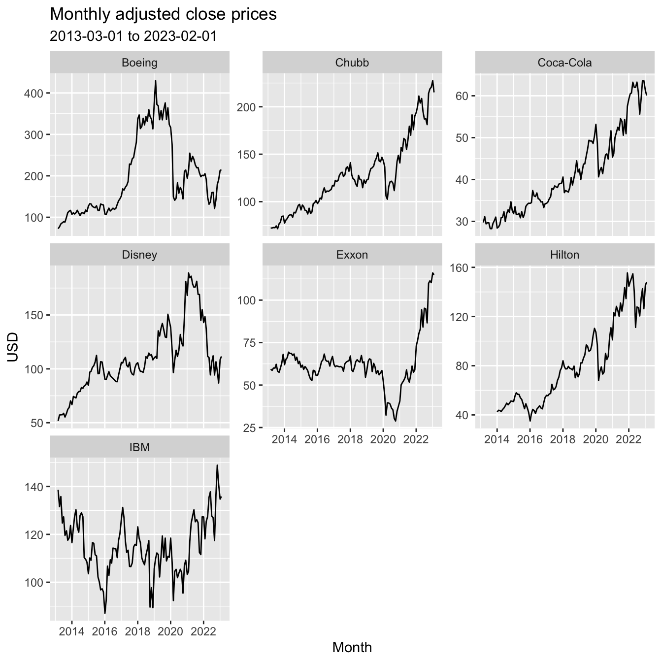
The historical data shows how the different companies/ sectors were impacted by Covid in early 2020 and the start of the Ukraine war in early 2022.
Plotting the monthly returns of each stock suggest that the assumption of a multivariate Normal distribution as a likelihood distribution is not too far fetched (alternatively we could look at log-returns, but it makes little difference here).
ggpairs(adj_returns[,-1],
         lower = list(continuous = wrap("points", alpha = 0.3, size=1),
              combo = wrap("dot", alpha = 0.4, size=0.2)))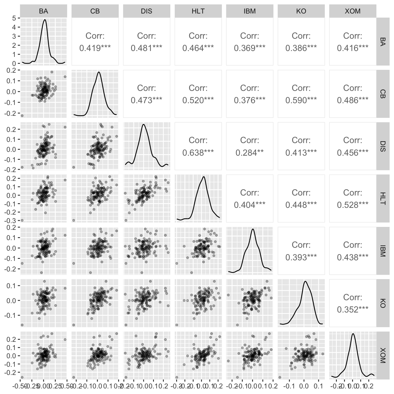
Next we look at the rolling 5 year window of monthly average returns and volatility. This highlights the challenge in deriving estimates for \(\mu_0\) and \(\Sigma\).
annualised_mean <- function(x){
  (1 + mean(x))^12 - 1
}
rolling_5yr_dt <- na.omit(price_dt[ , .(
  end_date = zoo::as.Date(frollapply(ref_date, 5*12, max)),
  rolling_5_yr_mean = frollapply(ret_adjusted_prices, 5*12, annualised_mean),
  rolling_5_yr_sd = frollapply(ret_adjusted_prices, 5*12, sd)*sqrt(12)
  ), by = comp_name])

ggplot(rolling_5yr_dt,
       aes(y = rolling_5_yr_mean,
           x = rolling_5_yr_sd,
           col = end_date)) +
  labs(
    title = "Rolling 5 year adjusted close price returns",
    x = "Rolling 5 year SD (%)",
    y = "Rolling 5 year mean (%)") +
  geom_point() +
  scale_y_continuous(labels = scales::percent) +
  scale_x_continuous(labels = scales::percent)  +
  guides(col=guide_legend(title="End date")) +
facet_wrap(~comp_name) 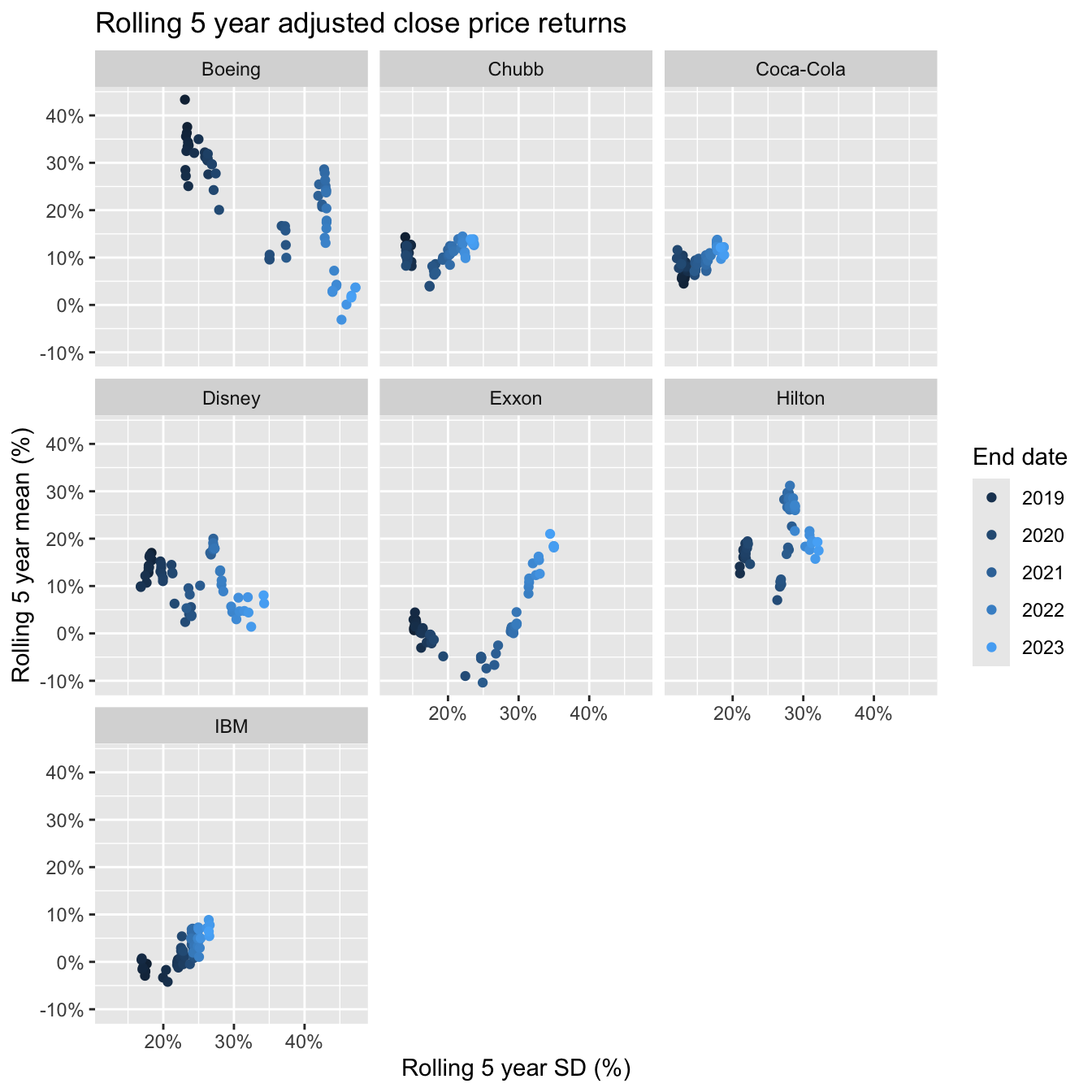
Given the volatility over the past few years it is not surprising that we see a drift in the scatter plots to the right. Unfortunately, the returns didn’t drift upwards for all companies. But that’s the past. We have to think about the future. To estimate the covariance matrix and excess equilibrium return we shall use the last 5 year window and assume a risk free rate of 3.5%. We will take a little short cut here and assume monthly re-weighting to today’s market cap weights.
start_date <- Sys.Date() - 5*365
rf <- 3.5/100 # Risk free rate assumption
# Estimate annualised covariance from historical monthly data
Sigma <- cov(adj_returns[ref_date >= start_date, -1]) * 12
round(Sigma,3)
## BA CB DIS HLT IBM KO XOM
## BA 0.300 0.071 0.115 0.106 0.066 0.062 0.106
## CB 0.071 0.076 0.058 0.064 0.026 0.034 0.056
## DIS 0.115 0.058 0.155 0.115 0.035 0.040 0.083
## HLT 0.106 0.064 0.115 0.148 0.039 0.051 0.087
## IBM 0.066 0.026 0.035 0.039 0.063 0.034 0.052
## KO 0.062 0.034 0.040 0.051 0.034 0.045 0.038
## XOM 0.106 0.056 0.083 0.087 0.052 0.038 0.161corrplot(cov2cor(Sigma), method = "pie", title = "Correlation",
mar = c(.25, .1, 2.5, .1), tl.srt = 45, diag = FALSE, type = "upper")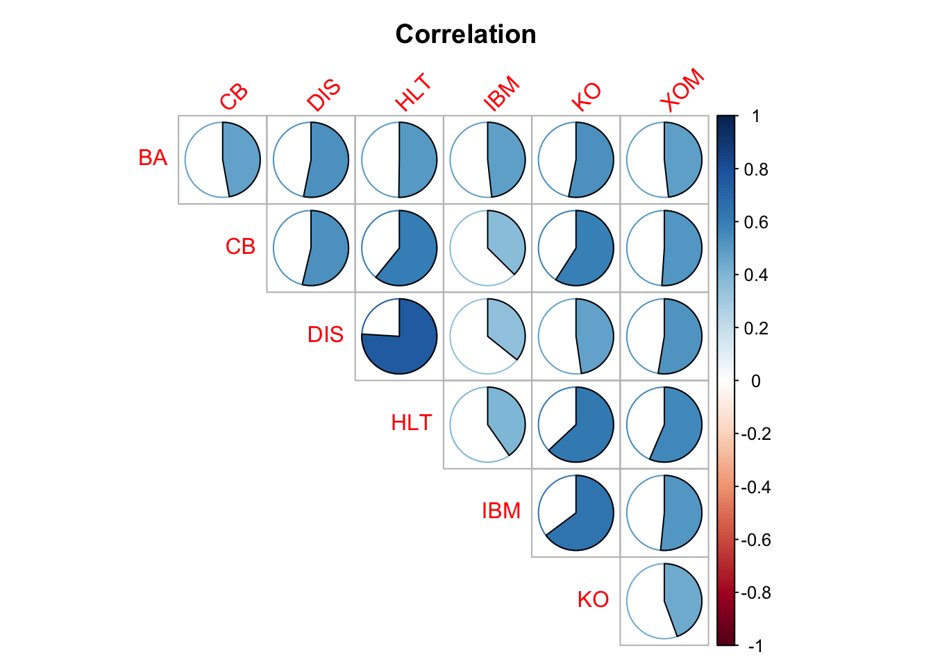
We set the parameter \(\tau\), which is linked to the uncertainty of the equilibrium excess returns, to 10%.
tau <- 0.1
# Estimate historical portfolio return
setkey(stock_dt, ticker)
setkey(comp_dt, ticker)
total_return <- price_dt[ref_date >= start_date, .(
  adj_ret = sum(ret_adjusted_prices * mkt_cap_weight)) ,
            by = ref_date]
# Estimate excess equilibrium returns by reverse optimisation
portfolio_mean_r <- annualised_mean(total_return$adj_ret)
portfolio_var <- var(total_return$adj_ret) * 12
lambda <- (portfolio_mean_r - rf)/portfolio_var
# Implied excess equilibrium returns
mu0 <- c(lambda) * (Sigma %*% mkt_cap_weight[colnames(Sigma)])

mu0_dt <- data.table(
  ticker,
  equilibrium_er = as.numeric(mu0),
  key = "ticker")

comp_mean_r_dt <- stock_dt[ref_date >= start_date, .(
  hist_5yr_mean_r = ((1 + mean(ret_adjusted_prices))^12-1)),
  keyby = ticker]

summary_dt <- comp_dt[comp_mean_r_dt][mu0_dt]| comp_name | ticker | mkt_cap_weight | hist_5yr_mean_r | equilibrium_er |
|---|---|---|---|---|
| Boeing | BA | 9.7% | 2.9% | 19.5% |
| Chubb | CB | 6.7% | 18.4% | 9.2% |
| Disney | DIS | 15.6% | 0.5% | 14.6% |
| Hilton | HLT | 3.1% | 19.5% | 14.3% |
| IBM | IBM | 9.6% | 7.7% | 8.1% |
| Coca-Cola | KO | 20.0% | 6.4% | 7.3% |
| Exxon | XOM | 35.3% | 39.3% | 17.4% |
Expert portfolio view
Let’s say, our expert believes Boeing will outperform Hilton by 5%, Disney’s return will be 1% higher than Coca-Cola and Exxon, and finally Chubb will outperform IBM and Coca-Cola by 3%.
We can capture this in the following pick matrix \(P\) and view vector \(q\). The uncertainties of our expert have been recorded in the \(\Omega\) matrix.
nViews <- 3
P <- matrix(
  c(1, 0, 0, -1, 0, 0, 0,
    0, 0, 1, 0, 0, -0.5, -0.5,
    0, 1, 0, 0, -0.5, -0.5, 0),
  nrow = nViews, byrow = TRUE
)
q <- c(0.05, 0.01, 0.03)
Omega <- (P %*% Sigma %*% t(P))
Black-Litterman model calculations
We have all the information required for the Black-Litterman formula:
K <- Sigma %*% t(P) %*% solve(tau * P %*% Sigma %*% t(P) + Omega)
# Estimate of mean Black-Litterman excess return
BL_mean_er <- mu0 + tau * K %*% (q - P %*% mu0)
# Estimate of the uncertainty for the BL excess returns
BL_Sigma <- tau * (Sigma - tau * K %*% P %*% Sigma)
## BL portfolio weights
BL_weight <- solve(Sigma) %*% BL_mean_er / lambda
## Posterior predictive covariance
BL_Sigma_Portfolio <- Sigma + BL_Sigma
summary_dt[, BL_mean_er := BL_mean_er]
summary_dt[, BL_weight := BL_weight]| comp_name | mkt_cap_weight | BL_weight | equilibrium_er | BL_mean_er |
|---|---|---|---|---|
| Boeing | 9.7% | 9.6% | 19.5% | 19.4% |
| Chubb | 6.7% | 8.3% | 9.2% | 9.3% |
| Disney | 15.6% | 14.7% | 14.6% | 14.5% |
| Hilton | 3.1% | 3.1% | 14.3% | 14.3% |
| IBM | 9.6% | 8.8% | 8.1% | 8.0% |
| Coca-Cola | 20.0% | 19.7% | 7.3% | 7.3% |
| Exxon | 35.3% | 35.8% | 17.4% | 17.4% |
Our expert’s positive outlook on Boeing and Chubb has tilted the portfolio weights in their favour, but not for Disney.
with(summary_dt,
     barplot(t(cbind(equilibrium_er,
                     BL_mean_er)) * 100,
             ylim = c(0, 15),
             beside = TRUE, names.arg = comp_name,
             legend = c("Equilibrium excess return",
                        "BL excess return"),
             border = NA, ylab = "Excess return (%)",
             args.legend = list(bty = "n")))
title("Excess returns", adj = 0)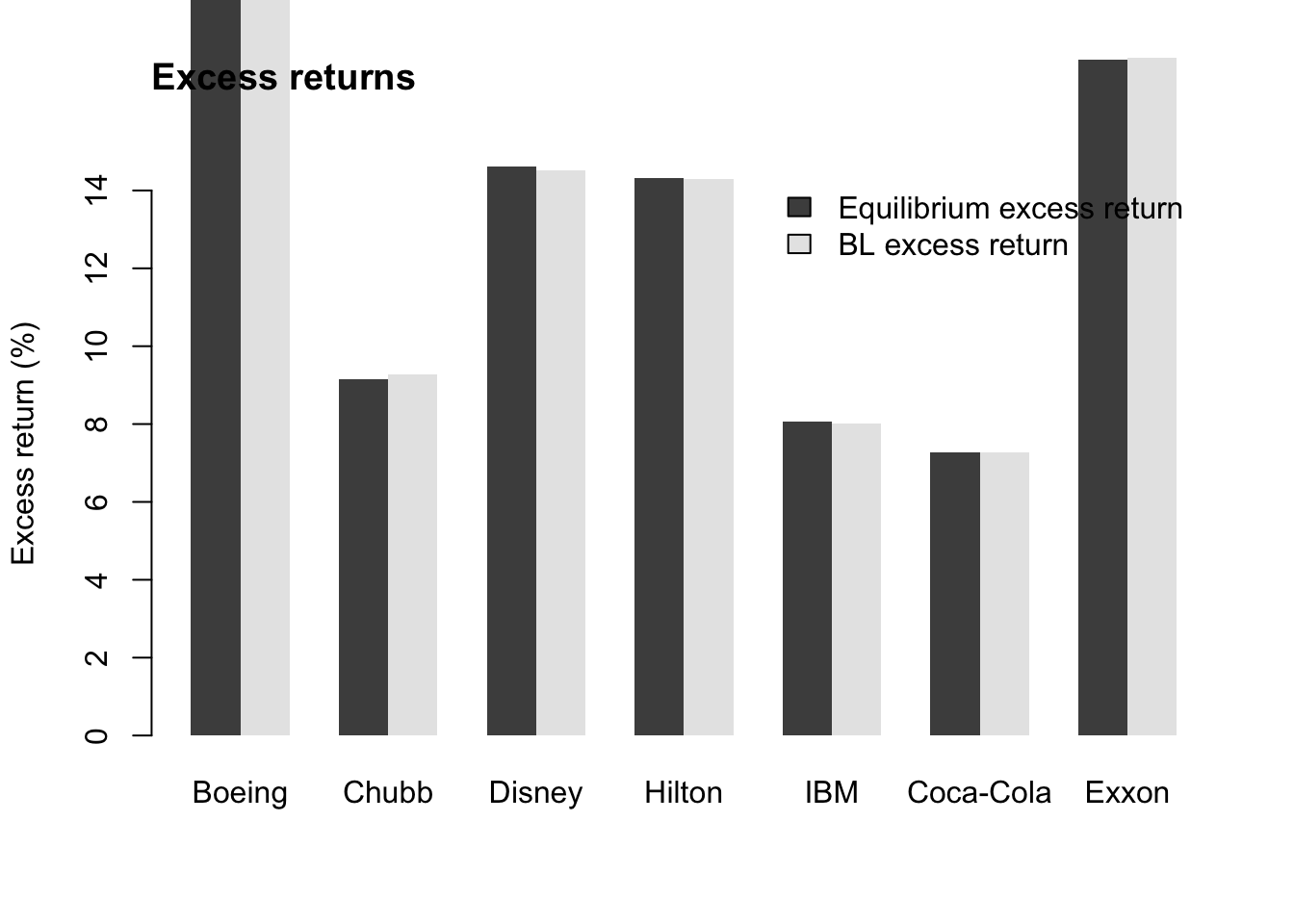
with(summary_dt,
     barplot(t(cbind(mkt_cap_weight,
                     BL_weight) * 100),
             ylim = c(0, 45),
             beside = TRUE, names.arg = comp_name,
             legend = c("Mkt cap weight", "BL weight"),
             border = NA, ylab = "Portfolio weight (%)",
             args.legend = list( bty = "n")))
title("Portfolio weights", adj = 0)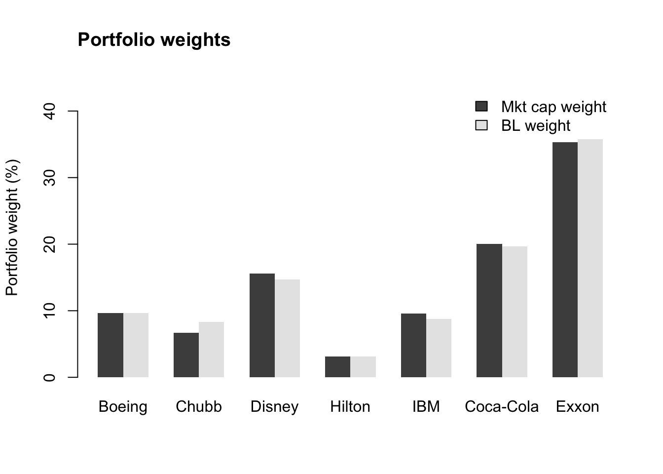
Although our expert’s views didn’t change the expected excess returns much, we can see that they did have an impact on the portfolio weights.
Posterior predictive returns
Now we can run posterior predictive simulations for the portfolio returns.
nSims <- 1e5
sample_rt <- mvrnorm(nSims, BL_mean_er, BL_Sigma_Portfolio)
sample_rt_portfolio <- as.numeric(sample_rt %*% BL_weight)
Let’s compare the historical 5 year rolling portfolio performance with the simulated 5 year rolling performance.
past_returns <- price_dt[, .(
  adj_ret = sum(ret_adjusted_prices * mkt_cap_weight)) ,
            by = ref_date]
past_rolling_5_yr <- na.omit(past_returns[ ,.(
  end_date = zoo::as.Date(frollapply(ref_date, 5*12, max)),
  rolling_5_yr_mean = frollapply(adj_ret, 5, annualised_mean),
  rolling_5_yr_sd =  frollapply(adj_ret, 5, sd)*sqrt(12)
)])
bl_sims_rolling_5_yr <- na.omit(data.table(
  rolling_5_yr_mean = frollapply(sample_rt_portfolio, 5, mean),
  rolling_5_yr_sd = frollapply(sample_rt_portfolio, 5, sd)
))
ggplot(past_rolling_5_yr, aes(
  x = rolling_5_yr_sd,
  y = rolling_5_yr_mean
)) + geom_point() +
  geom_density_2d(data = bl_sims_rolling_5_yr,
                  aes(x = rolling_5_yr_sd,
                      y = rolling_5_yr_mean)) +
  labs(
    title = "Rolling 5 year monthly adjusted returns vs. simulated future performance",
    subtitle = paste("Data used (black dots):",
                     min(past_returns$ref_date), "to",
                    max(past_returns$ref_date)),
    x = "Rolling 5 year SD (%)",
    y = "Rolling 5 year mean (%)") +
  scale_y_continuous(labels = scales::percent) +
  scale_x_continuous(labels = scales::percent)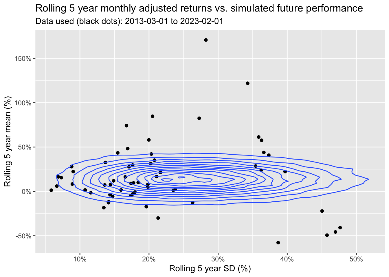
Perhaps, the model/ view is a little off target? But how representative is the past of future performance? Past performance is no guarantee of future results. That’s the beauty of the Black-Litterman model, as it allows us to incorporate experts’ views of the future.
However, what I find most fascinating is the creative approach of incorporating expert’s views on absolute and relative performance and treating them as observations, while what might be seen as data, i.e., market data, is treated as prior information.
Session Info
session_info <- (sessionInfo()[-8])
utils:::print.sessionInfo(session_info, local=FALSE)
## R version 4.4.2 (2024-10-31)
## Platform: aarch64-apple-darwin20
## Running under: macOS Sequoia 15.2
##
## Matrix products: default
## BLAS: /Library/Frameworks/R.framework/Versions/4.4-arm64/Resources/lib/libRblas.0.dylib
## LAPACK: /Library/Frameworks/R.framework/Versions/4.4-arm64/Resources/lib/libRlapack.dylib; LAPACK version 3.12.0
##
## attached base packages:
## NULL
##
## other attached packages:
## [1] corrplot_0.95 MASS_7.3-61 gt_0.11.1 GGally_2.2.1
## [5] scales_1.3.0 ggplot2_3.5.1 zoo_1.8-12 data.table_1.16.4
## [9] yfR_1.1.0
##
## loaded via a namespace (and not attached):
## [1] sass_0.4.9 generics_0.1.3 tidyr_1.3.1 xml2_1.3.6
## [5] blogdown_1.19 lattice_0.22-6 digest_0.6.37 magrittr_2.0.3
## [9] evaluate_1.0.1 grid_4.4.2 RColorBrewer_1.1-3 bookdown_0.41
## [13] fastmap_1.2.0 plyr_1.8.9 jsonlite_1.8.9 purrr_1.0.2
## [17] isoband_0.2.7 jquerylib_0.1.4 cli_3.6.3 rlang_1.1.4
## [21] munsell_0.5.1 withr_3.0.2 cachem_1.1.0 yaml_2.3.10
## [25] tools_4.4.2 dplyr_1.1.4 colorspace_2.1-1 ggstats_0.7.0
## [29] vctrs_0.6.5 R6_2.5.1 lifecycle_1.0.4 pkgconfig_2.0.3
## [33] pillar_1.10.0 bslib_0.8.0 gtable_0.3.6 glue_1.8.0
## [37] Rcpp_1.0.13-1 xfun_0.49 tibble_3.2.1 tidyselect_1.2.1
## [41] rstudioapi_0.17.1 knitr_1.49 farver_2.1.2 htmltools_0.5.8.1
## [45] rmarkdown_2.29 labeling_0.4.3 compiler_4.4.2References
Citation
For attribution, please cite this work as:Markus Gesmann (Feb 15, 2023) Portfolio Allocation for Bayesian Dummies. Retrieved from https://magesblog.com/post/2023-02-15-portfolio-allocation-for-bayesian-dummies/
@misc{ 2023-portfolio-allocation-for-bayesian-dummies,
author = { Markus Gesmann },
title = { Portfolio Allocation for Bayesian Dummies },
url = { https://magesblog.com/post/2023-02-15-portfolio-allocation-for-bayesian-dummies/ },
year = { 2023 }
updated = { Feb 15, 2023 }
}