Case study

Suppose we have a process that can be described by a parametric non-linear growth curve, say a Weibull CDF:

\[ \begin{aligned} g(t; \lambda, k) & = 1 - e^{-(t/\lambda)^k} \end{aligned} \]

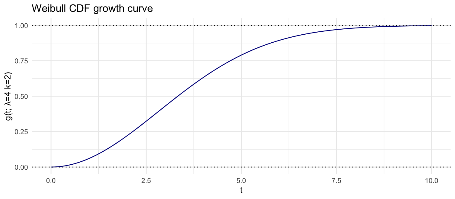
Since the curve converges to an ‘ultimate’ position of 100% the variance of the data will shrink from one measurement to the next. Indeed, the incremental change will converge to 0 as time progresses.

Hence, modelling a constant variance makes little sense, but a constant coefficient of variation is not unreasonable, if applied to the incremental data.

To illustrate the point let’s simulate data using a log-normal measurement distribution with a constant sdlog parameter over time, i.e. a constant coefficient of variation.

The following code snippet simulates 20 Weibull growth curves on a cumulative and incremental basis. The incremental simulations are then aggregated to be compared with the cumulative simulations.

# Parameters
nSims <- 20
dt <- 0.1
time <- seq(0, 10, dt)
lambda <- 4; k <- 2
sdlog <- 0.5

t <- rep(time, nSims)
N <- length(t); 
g <- function(t, lambda, k){
  (1 - exp(-(t /lambda)^k))
}
# Simulations
set.seed(1234)
sim_cumulative <- rlnorm(N, log(g(t, lambda, k)), sdlog)
set.seed(1234)
sim_incremental <-  rlnorm(N, ifelse(
  t > dt, log(g(t, lambda, k) - g(t - dt, lambda, k)),
             log(g(t, lambda, k))), sdlog)

# Visualisation
library(latticeExtra)
library(data.table)

Sims <- data.table(SimID = rep(1:nSims, each = length(time)), 
                   sim_cumulative, sim_incremental)  
Sims[, `cumsum(sim_incremental)` := cumsum(sim_incremental), by=SimID]

xyplot(sim_cumulative + sim_incremental + `cumsum(sim_incremental)` ~ t,
       groups = SimID, data = Sims,
       ylab ="", xlab = "time",
       t="l", col=adjustcolor(1:nSims, alpha.f = 0.25),
       main = paste("Illustration of modelling cumulative vs incremental growth",
                    "20 simulations with a log-normal distribution", sep="\n"),
       scale= "free", layout = c(3, 1),
       par.settings = theEconomist.theme())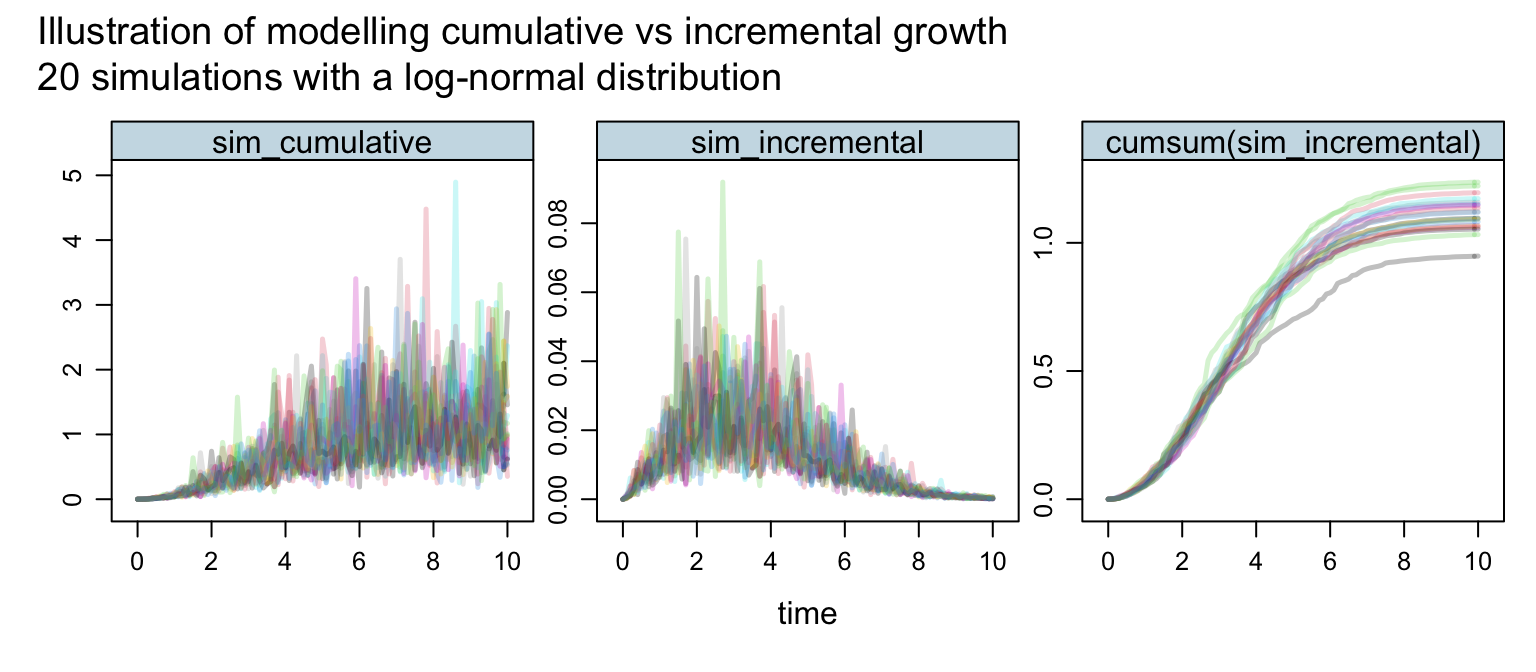

The first plot illustrates nicely that modelling growth data on a cumulative basis with a fixed coefficient of variance results in unrealistic simulations - the volatility increases as the growth reaches its maturity level. The plot on the right looks a lot more like real data. In particular given that all incremental simulations are either zero or positive we end up with monotone increasing curves when those simulations are aggregated over time. That’s what we observe in most growth data, e.g. think again of the growth development of children, or claims payments in the context of insurance.

Additional factors which favour the use of incremental data include the following:

• Missing or corrupted data for some development periods can be problematic when we require cumulative data from the underlying incremental cash flows. Manual interpolation techniques can be used ahead of modelling, but a parametric growth curve applied to incremental data will deal with missing data as part of the modelling process.
• Changes in underlying processes (claims handling or inflation) causing effects in the calendar period dimension can be masked in cumulative data and are easier to identify and model using incremental data.
• Predictions of future payments are put on an additive scale, rather than a multiplicative scale, which avoids ad hoc anchoring of future claims projections to the latest cumulative data point.

For more details read section 3.3 of our paper.

Session Info

session_info <- (sessionInfo()[-8])
utils:::print.sessionInfo(session_info, local=FALSE)

## R version 4.1.1 (2021-08-10)
## Platform: aarch64-apple-darwin20 (64-bit)
## Running under: macOS Big Sur 11.5.1
## 
## Matrix products: default
## BLAS:   /Library/Frameworks/R.framework/Versions/4.1-arm64/Resources/lib/libRblas.0.dylib
## LAPACK: /Library/Frameworks/R.framework/Versions/4.1-arm64/Resources/lib/libRlapack.dylib
## 
## attached base packages:
## [1] stats     graphics  grDevices utils     datasets  methods   base     
## 
## other attached packages:
## [1] data.table_1.14.0   latticeExtra_0.6-29 lattice_0.20-44    
## [4] ggplot2_3.3.5