Prediction for the 100m final at the Tokyo Olympics
On Sunday the Tokyo Olympics men sprint 100m final will take place. Francesc Montané reminded me in his analysis that 9 years ago I used a simple regression model to predict the winning time for the 100m men sprint final of the 2012 Olympics in London. My model predicted a winning time of 9.68s, yet Usain Bolt finished in 9.63s. For this Sunday my prediction is 9.72s, with a 50% credible interval of [9.60s, 9.84s].
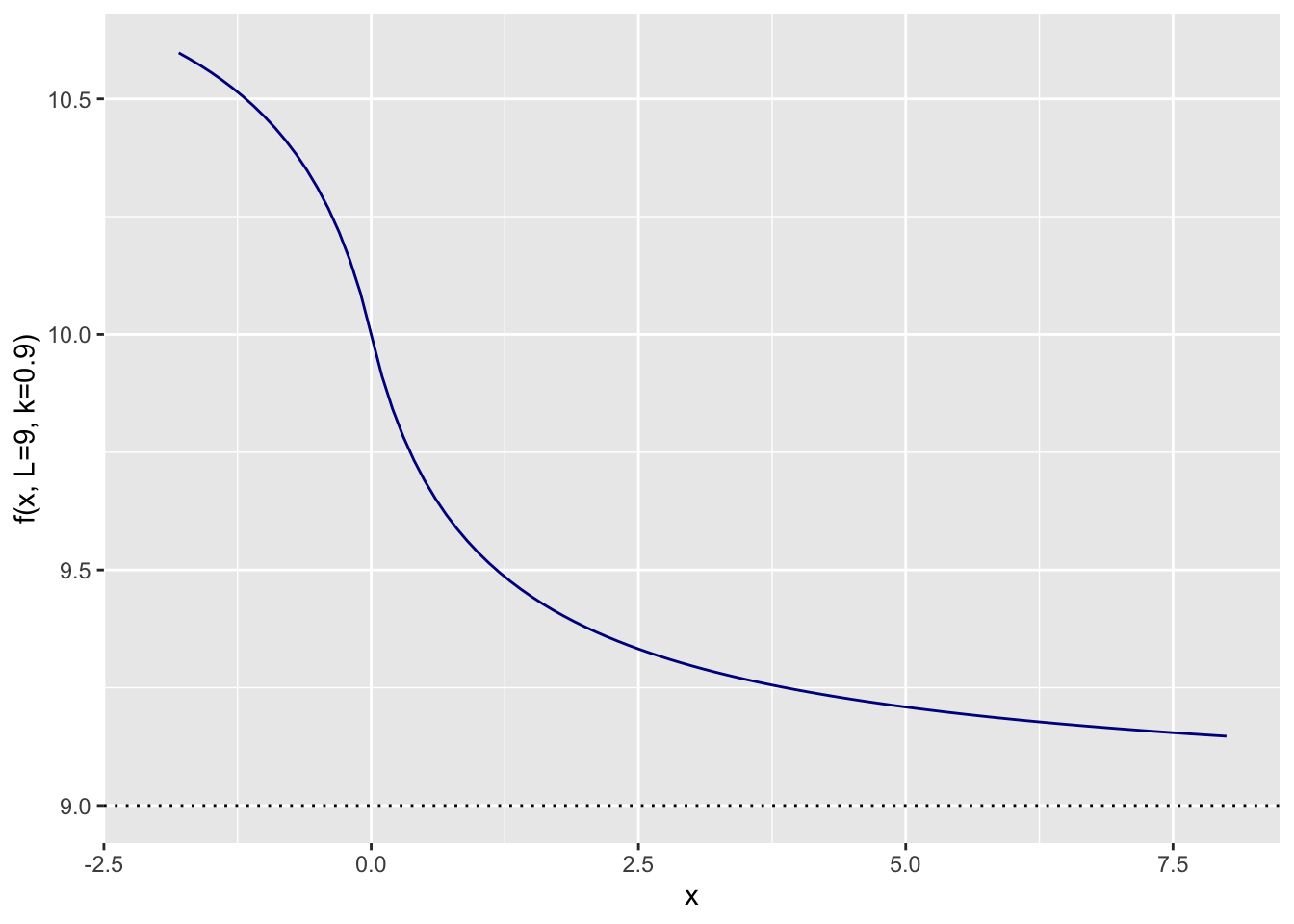
Since the 2012 Olympics many things have changed; Usain Bolt has retired and new shoes with advance spike technology have created a little bit of a controversy. Reviewing my old model, I don’t think a log-linear regression is still sensible. We may see faster times, but there will be a limit. Hence, an S-shape curve might be a good starting point. There are many to choose from. I picked the following that converges to \(L\):
\[ \begin{aligned} f(x) = & L + 1 - \frac{x}{\left(1 + |x|^{k}\right)^{1/k}} \\ \end{aligned} \]
With \(L=9\) and \(k=0.9\) it looks like this:
Data
Here is the historical data of the Gold medal winning time again:
library(data.table)
golddata <- fread(
  sep=",", header=TRUE,
  text="
  Year, Event, Athlete, Medal, Country, Time
1896, 100m Men,        Tom Burke,  GOLD,     USA,  12.00
1900, 100m Men,     Frank Jarvis,  GOLD,     USA,  11.00
1904, 100m Men,      Archie Hahn,  GOLD,     USA,  11.00
1906, 100m Men,      Archie Hahn,  GOLD,     USA,  11.20
1908, 100m Men,    Reggie Walker,  GOLD,     SAF,  10.80
1912, 100m Men,      Ralph Craig,  GOLD,     USA,  10.80
1920, 100m Men,  Charles Paddock,  GOLD,     USA,  10.80
1924, 100m Men,  Harold Abrahams,  GOLD,     GBR,  10.60
1928, 100m Men,   Percy Williams,  GOLD,     CAN,  10.80
1932, 100m Men,      Eddie Tolan,  GOLD,     USA,  10.30
1936, 100m Men,      Jesse Owens,  GOLD,     USA,  10.30
1948, 100m Men, Harrison Dillard,  GOLD,     USA,  10.30
1952, 100m Men,   Lindy Remigino,  GOLD,     USA,  10.40
1956, 100m Men,     Bobby Morrow,  GOLD,     USA,  10.50
1960, 100m Men,       Armin Hary,  GOLD,     GER,  10.20
1964, 100m Men,        Bob Hayes,  GOLD,     USA,  10.00
1968, 100m Men,        Jim Hines,  GOLD,     USA,   9.95
1972, 100m Men,    Valery Borzov,  GOLD,     URS,  10.14
1976, 100m Men,  Hasely Crawford,  GOLD,     TRI,  10.06
1980, 100m Men,      Allan Wells,  GOLD,     GBR,  10.25
1984, 100m Men,       Carl Lewis,  GOLD,     USA,   9.99
1988, 100m Men,       Carl Lewis,  GOLD,     USA,   9.92
1992, 100m Men, Linford Christie,  GOLD,     GBR,   9.96
1996, 100m Men,   Donovan Bailey,  GOLD,     CAN,   9.84
2000, 100m Men,   Maurice Greene,  GOLD,     USA,   9.87
2004, 100m Men,    Justin Gatlin,  GOLD,     USA,   9.85
2008, 100m Men,       Usain Bolt,  GOLD,     JAM,   9.69
2012, 100m Men,       Usain Bolt,  GOLD,     JAM,   9.63
2016, 100m Men,       Usain Bolt,  GOLD,     JAM,   9.81
")
library(ggplot2)
ggplot(golddata, aes(x=Year, y=Time)) +
geom_line() + geom_point() +
labs(title="Winning times of Olympic gold medalist 100m sprint men")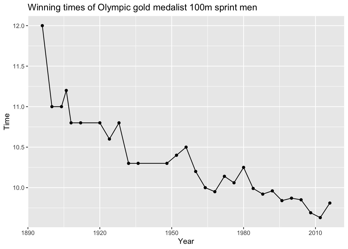
Model
First I prepare the data, I remove the first measurement from 1896 that looks too much like an outlier. To fit the non-linear function it is helpful to centre and scale the ‘Year’ metric. However, instead of doing this right away, I will include variables ‘C’ (centre) and ‘S’ (scale) in my model.
golddata1900 <- golddata[Year>=1900]
c(C = mean(golddata1900$Year),
  S = sd(golddata1900$Year))
## C S
## 1958.78571 36.69833For my Bayesian regression model I assume a Normal (aka Gaussian) data distribution and Normal priors for the parameters:
\[
\begin{aligned}
\mathsf{Time} \sim & \mathsf{Normal}(f(\mathsf{Year}, C, S, L, k), \sigma) \\
f(\mathsf{Year}, C, S, L, k) = & L + 1 - \frac{(\mathsf{Year}-C)/S}{\left(1 + |(\mathsf{Year}-C)/S|^{k}\right)^{1/k}} \\
C\sim & \mathsf{Normal}(1959, 5) \\
S\sim & \mathsf{Normal}(37, 1) \\
L\sim & \mathsf{Normal}(9, 0.2) \\
k \sim & \mathsf{Normal}(1, 0.2)\\
\sigma \sim & \mathsf{StudentT}(3, 0, 2.5)
\end{aligned}
\]
To fit the non-linear function I use the brms package:
library(brms)
library(parallel)
nCores <- detectCores()
options(mc.cores = nCores)
mdl <- brm(
  bf(Time ~ L + 1 - ((Year-C)/S)/(1+fabs((Year-C)/S)^k)^(1/k),
     C ~ 1, S ~ 1, L ~ 1, k ~ 1, nl = TRUE),
  data = golddata1900, family = gaussian(),
  prior = c(
    prior(normal(1959, 5), nlpar = "C"),
    prior(normal(37, 1), nlpar = "S"),
    prior(normal(9, 0.2), nlpar = "L", lb=0),
    prior(normal(1, 0.2), nlpar = "k", lb=0),
    prior(student_t(3, 0, 2.5), class = "sigma")
  ),
  seed = 1234, iter = 2000,
  chains = 4, cores = nCores,
)mdl## Family: gaussian
## Links: mu = identity; sigma = identity
## Formula: Time ~ L + 1 - ((Year - C)/S)/(1 + fabs((Year - C)/S)^k)^(1/k)
## C ~ 1
## S ~ 1
## L ~ 1
## k ~ 1
## Data: golddata1900 (Number of observations: 28)
## Samples: 4 chains, each with iter = 2000; warmup = 1000; thin = 1;
## total post-warmup samples = 4000
##
## Population-Level Effects:
## Estimate Est.Error l-95% CI u-95% CI Rhat Bulk_ESS Tail_ESS
## C_Intercept 1956.62 4.17 1947.95 1964.53 1.00 2403 2066
## S_Intercept 37.12 1.00 35.18 39.10 1.00 2770 2547
## L_Intercept 9.31 0.05 9.21 9.40 1.00 2483 2388
## k_Intercept 0.90 0.09 0.74 1.10 1.00 3803 2643
##
## Family Specific Parameters:
## Estimate Est.Error l-95% CI u-95% CI Rhat Bulk_ESS Tail_ESS
## sigma 0.18 0.03 0.13 0.24 1.00 3269 2478
##
## Samples were drawn using sampling(NUTS). For each parameter, Bulk_ESS
## and Tail_ESS are effective sample size measures, and Rhat is the potential
## scale reduction factor on split chains (at convergence, Rhat = 1).The model runs without problems and the estimated parameters are not too far away from my prior assumptions. Nice!
The parameter \(L\) represents the fastest a human could possibly run. The 95% credible interval is between 9.21s and 9.40s.
Plotting the fitted model with the 95% credible interval demonstrates that it captures the observations well:
plot(brms::conditional_effects(mdl, method = "predict", prob=0.95), points=TRUE)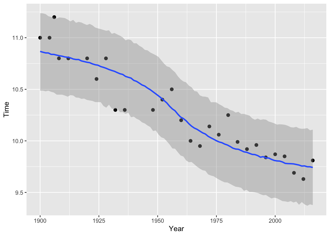
Prediction
The model looks plausible, so what are the predictions for this Sunday, and the Olympics in Paris and Los Angeles?
p <- brms::posterior_predict(
  mdl, newdata=data.frame(Year=c(2021, 2024, 2028)))
colnames(p) <- c(2021, 2024, 2028)
rbind(
  mean=apply(p, 2, mean),
  apply(p, 2, quantile, probs=c(0.25, 0.5, 0.75))
)
## 2021 2024 2028
## mean 9.722309 9.712602 9.698752
## 25% 9.603301 9.593783 9.574987
## 50% 9.724628 9.714867 9.698922
## 75% 9.843578 9.837005 9.824547A winning time of close to 9.72s for this Sunday might be achievable. But the fastest time this year, of the American Trayvon Bromell, who is favourite to take Bolt’s 100m title in Tokyo, was 9.77s.
Interestingly, Francesc’s ETS model without Usain Bolt’s data is predicting a winning time of 9.73s.
Session Info
utils:::print.sessionInfo(sessionInfo()[-8], local=FALSE)## R version 4.1.0 (2021-05-18)
## Platform: aarch64-apple-darwin20 (64-bit)
## Running under: macOS Big Sur 11.5.1
##
## Matrix products: default
## BLAS: /Library/Frameworks/R.framework/Versions/4.1-arm64/Resources/lib/libRblas.dylib
## LAPACK: /Library/Frameworks/R.framework/Versions/4.1-arm64/Resources/lib/libRlapack.dylib
##
## attached base packages:
## [1] parallel stats graphics grDevices utils datasets methods
## [8] base
##
## other attached packages:
## [1] brms_2.15.0 Rcpp_1.0.7 data.table_1.14.0 ggplot2_3.3.5Citation
For attribution, please cite this work as:Markus Gesmann (Jul 29, 2021) Prediction for the 100m final at the Tokyo Olympics. Retrieved from https://magesblog.com/post/2021-07-29-prediction-for-the-100m-tokyo-olympics/
@misc{ 2021-prediction-for-the-100m-final-at-the-tokyo-olympics,
author = { Markus Gesmann },
title = { Prediction for the 100m final at the Tokyo Olympics },
url = { https://magesblog.com/post/2021-07-29-prediction-for-the-100m-tokyo-olympics/ },
year = { 2021 }
updated = { Jul 29, 2021 }
}