Use domain knowledge to review prior distributions
At the Insurance Data Science conference, both Eric Novik and Paul-Christian Bürkner emphasised in their talks the value of thinking about the data generating process when building Bayesian statistical models. It is also a key step in Michael Betancourt’s Principled Bayesian Workflow.
In this post, I will discuss in more detail how to set priors, and review the prior and posterior parameter distributions, but also the prior predictive distributions with brms (Bürkner (2017)).
The prior predictive distribution shows me how the model behaves before I use my data. Thus, I can check if the model describes the data generating process reasonably well, before I go through the lengthy process of fitting the model.
As an example, I will get back to the non-linear hierarchical growth curve model, which is also part of the brms package vignette on non-linear models.
Load packages and data
First I load the relevant packages and data set.
library(rstan)
library(brms)
library(bayesplot)
rstan_options(auto_write = TRUE)
options(mc.cores = parallel::detectCores())
theme_update(text = element_text(family = "sans"))
library(data.table)
url <- "https://raw.githubusercontent.com/mages/diesunddas/master/Data/ClarkTriangle.csv"
loss <- fread(url)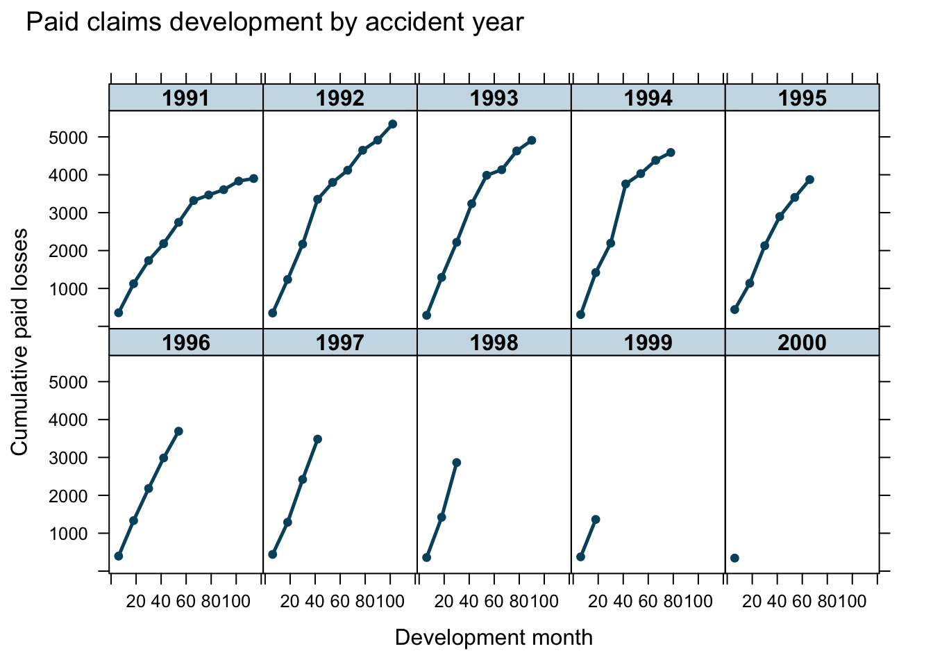
It is the aim to use growth curves to model the claims payments of insurance losses from different accident years (1991 - 2000) over time (development months) and predict future payments.
Prior predictive distribution
I will start with the same model as in the brms vignette, but instead of fitting the model, I set the parameter sample_prior = "only" to generate samples from the prior predictive distribution only, i.e. the data will be ignored and only the prior distributions will be used.
nlform1 <- bf(cum ~ ult * (1 - exp(-(dev/theta)^omega)),
             ult ~ 1 + (1|AY), omega ~ 1, theta ~ 1,
             nl = TRUE)
m1 <- brm(nlform1, data = loss, family = gaussian(),
  prior = c(
    prior(normal(5000, 1000), nlpar = "ult"),
    prior(normal(1, 2), nlpar = "omega"),
    prior(normal(45, 10), nlpar = "theta")
  ),
  sample_prior = "only", seed = 1234,
  control = list(adapt_delta = 0.9)
)
I can use the same plots to review the prior predictive distribution as I would have done for the posterior predictive distribution.
conditions <- data.frame(AY = unique(loss$AY))
rownames(conditions) <- unique(loss$AY)
me_loss_prior1 <- marginal_effects(
  m1, conditions = conditions,
  re_formula = NULL, method = "predict"
)
p0 <- plot(me_loss_prior1, ncol = 5, points = TRUE, plot = FALSE)
p0$dev + ggtitle("Prior predictive distributions")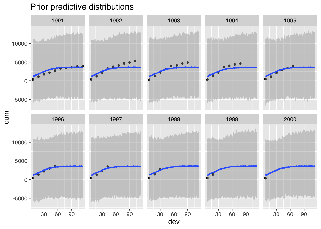
Perhaps this doesn’t look too bad, but the model generates also many negative claims payments, as I have assumed a Gaussian distribution. Yet, customers rarely pay claims back to the insurance company.
In addition, this model simplifies the variance structure to a constant \(\sigma^2\). In (Guszcza (2008)) Jim Guszcza suggested a variance that is proportional to the claims amount.
Review model code and priors
Let’s look at a part of the brm-generated Stan code that describes the priors to better understand the model:
  // priors including all constants
  target += normal_lpdf(b_ult | 5000, 1000);
  target += normal_lpdf(b_omega | 1, 2);
  target += normal_lpdf(b_theta | 45, 10);
  target += student_t_lpdf(sigma | 3, 0, 1964)
    - 1 * student_t_lccdf(0 | 3, 0, 1964);
  target += student_t_lpdf(sd_1 | 3, 0, 1964)
    - 1 * student_t_lccdf(0 | 3, 0, 1964);
  target += normal_lpdf(z_1[1] | 0, 1);
  // likelihood including all constants
  if (!prior_only) {
    target += normal_lpdf(Y | mu, sigma);
  }
The code shows the default priors set by brm for sigma and sd_1, which I didn’t set explicitly. In addition, the last line shows the switch that turns off sampling from the posterior distributions.
Putting the model in ‘Greek’ makes it more readable:
\[ \begin{align} loss_{AY}(t) & \sim \mathcal{N}\left( \mu_{AY}(t), \sigma^2\right) \\ \mu_{AY}(t) & = \gamma_{AY} \cdot G(t; \omega, \theta)\\ G(t; \omega, \theta) & = 1 - \exp\left(-\left({t/\theta}\right)^\omega\right)\\ \gamma_{AY} & = \gamma + \gamma_{AY}^0 \\ \mbox{Priors}&:\\ \gamma & \sim \mathcal{N}(5000, 1000)\\ \omega & \sim \mathcal{N}\left(1, 2^2\right)\\ \theta & \sim \mathcal{N}\left(45, 10^2\right) \\ \sigma & \sim \mbox{Student-t}\left(3, 0, 1964\right)^+\\ \gamma_{AY}^0 & \sim \mathcal{N}(0, \sigma_{\gamma^0}^2) \\ \sigma_{\gamma^0} & \sim \mbox{Student-t}\left(3, 0, 1964\right)^+\\ \end{align} \]
Utilise domain knowledge
There are a few aspects that I would like to change to the original model:
- Use the loss ratio instead of the loss amounts to make data from the different years more comparable and to bring values closer to 1
- Change the distribution family from Gaussian to lognormal to avoid negative payments being generated
- Assume a constant \(\sigma\) parameter, which means a constant coefficient of variation in case of the lognormal distribution, i.e. the standard deviation is proportional to the mean
- Use development year instead of development month to reduce the scale of \(t\)
- Use parameter \(\phi=1/\theta\), since I believe \(0< \phi < 1\).
- Shrink uncertainty and shift \(\omega\), as I believe \(\omega\) will be around 1.25
- With the move to loss ratios the standard deviations \(\sigma_{\gamma^0}\) and \(\sigma\) will be much smaller. Therefore, I reduce the scale parameter and increase the degrees of freedoms from 3 to 5 for the Student-t distribution
My new model looks like this now:
\[ \begin{align} \ell_{AY}(t) & \sim \log \mathcal{N}\left(\log(\mu_{AY}(t)), \sigma^2\right) \\ \mu_{AY}(t) & = \gamma_{AY} \cdot G(t; \omega, \phi)\\ G(t;\omega, \phi) & = 1 - \exp\left(-\left(t\cdot \phi\right)^\omega\right)\\ \gamma_{AY} & = \gamma + \gamma_{AY}^0 \\ \mbox{Priors}&:\\ \gamma & \sim \log \mathcal{N}\left(\log(0.5), \log(1.2)^2\right)\\ \omega & \sim \mathcal{N}\left(1.25, 0.25^2\right)^+\\ \phi & \sim \mathcal{N}\left(0.25, 0.25^2\right)^+ \\ \sigma & \sim \mbox{Student-t}\left(5, 0, 0.25\right)^+\\ \gamma_{AY}^0 & \sim \mathcal{N}(0, \sigma_{\gamma^0}^2) \\ \sigma_{\gamma^0} & \sim \mbox{Student-t}\left(5, 0, 0.25\right)^+\\ \end{align} \]
Assuming a constant coefficient of variation across development time seems broadly okay:
loss <- loss[, `:=`(loss_ratio = cum/loss$premium,
                    dev_year = (dev+6)/12)]
print(
  loss[, list(`CV(loss_ratio)` = sd(loss_ratio)/mean(loss_ratio)), by=dev_year],
  digits=1)
## dev_year CV(loss_ratio)
## 1: 1 0.14
## 2: 2 0.08
## 3: 3 0.08
## 4: 4 0.15
## 5: 5 0.13
## 6: 6 0.09
## 7: 7 0.11
## 8: 8 0.14
## 9: 9 0.21
## 10: 10 NATo review if my new model makes sense I start by generating samples from the priors again:
nlform2 <- bf(loss_ratio ~ log(ulr * (1 - exp(-(dev_year*phi)^omega))),
             ulr ~ 1 + (1|AY), omega ~ 1, phi ~ 1,
             nl = TRUE)
m2 <- brm(nlform2, data = loss,
  family = lognormal(link = "identity", link_sigma = "log"),
  prior = c(
    prior(lognormal(log(0.5), log(1.2)), nlpar = "ulr", lb=0),
    prior(normal(1.25, 0.25), nlpar = "omega", lb=0),
    prior(normal(0.25, 0.25), nlpar = "phi", lb=0),
    prior(student_t(5, 0, 0.25), class = "sigma"),
    prior(student_t(5, 0, 0.25), class = "sd", nlpar="ulr")
    ),
    sample_prior = "only", seed = 1234
)
Prior parameter distributions
library(bayesplot)
theme_update(text = element_text(family = "sans"))
mcmc_areas(
   as.array(m2),
   pars = c("b_ulr_Intercept", "b_omega_Intercept",
            "b_phi_Intercept",
            "sd_AY__ulr_Intercept", "sigma"),
   prob = 0.8, # 80% intervals
   prob_outer = 0.99, # 99%
   point_est = "mean"
) + ggplot2::labs(
  title = "Prior parameter distributions",
  subtitle = "with medians and 80% intervals"
)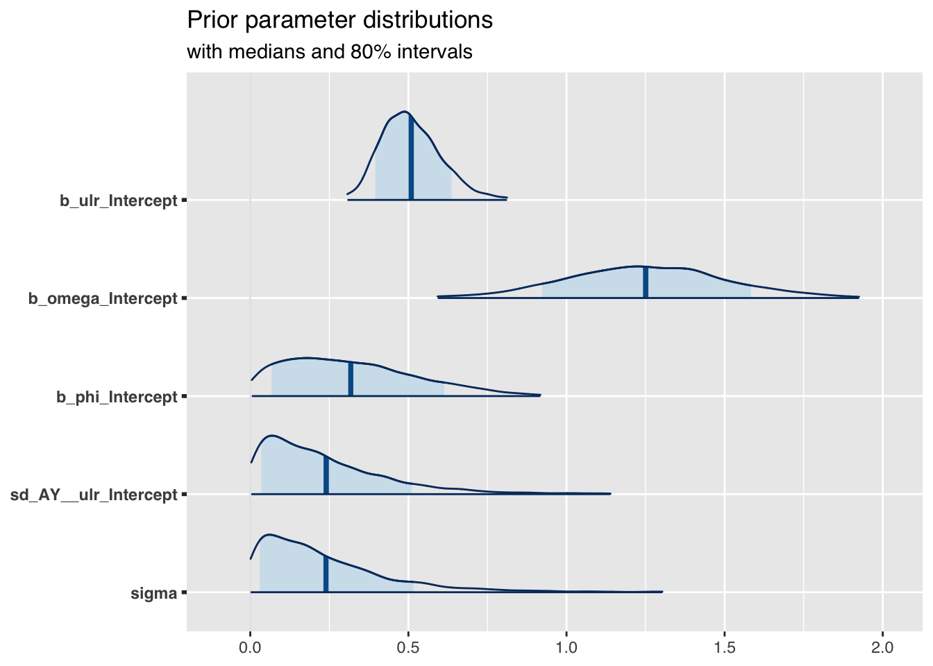
The prior parameter distributions look very similar to what I would expect, given the plot above.
Prior predictive distributions
me_loss_prior2 <- marginal_effects(
  m2, conditions = conditions,
  re_formula = NULL, method = "predict"
)
p1 <- plot(me_loss_prior2, ncol = 5, points = TRUE, plot = FALSE)
p1$dev + ggtitle("Prior predictive distributions")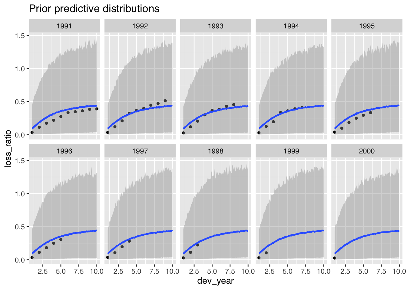
The prior predictive distributions look also more in line with the data.
I am happy with the model as it is. In my next step, I start using the data to fit the model.
Generate posterior samples
To fit my model with the data I call update and set the parameter sample_prior="no". Note, the model doesn’t need to be recompiled.
(fit_m1 <- update(m2, sample_prior="no", seed = 1234))## Family: lognormal
## Links: mu = identity; sigma = identity
## Formula: loss_ratio ~ log(ulr * (1 - exp(-(dev_year * phi)^omega)))
## ulr ~ 1 + (1 | AY)
## omega ~ 1
## phi ~ 1
## Data: loss (Number of observations: 55)
## Samples: 4 chains, each with iter = 2000; warmup = 1000; thin = 1;
## total post-warmup samples = 4000
##
## Group-Level Effects:
## ~AY (Number of levels: 10)
## Estimate Est.Error l-95% CI u-95% CI Rhat Bulk_ESS Tail_ESS
## sd(ulr_Intercept) 0.03 0.01 0.01 0.07 1.00 992 1500
##
## Population-Level Effects:
## Estimate Est.Error l-95% CI u-95% CI Rhat Bulk_ESS Tail_ESS
## ulr_Intercept 0.42 0.02 0.38 0.46 1.00 1676 2176
## omega_Intercept 1.86 0.05 1.76 1.95 1.00 2207 2575
## phi_Intercept 0.26 0.01 0.23 0.28 1.00 1985 2233
##
## Family Specific Parameters:
## Estimate Est.Error l-95% CI u-95% CI Rhat Bulk_ESS Tail_ESS
## sigma 0.10 0.01 0.08 0.13 1.00 2439 2434
##
## Samples were drawn using sampling(NUTS). For each parameter, Bulk_ESS
## and Tail_ESS are effective sample size measures, and Rhat is the potential
## scale reduction factor on split chains (at convergence, Rhat = 1).The model looks well behave at a first glance.
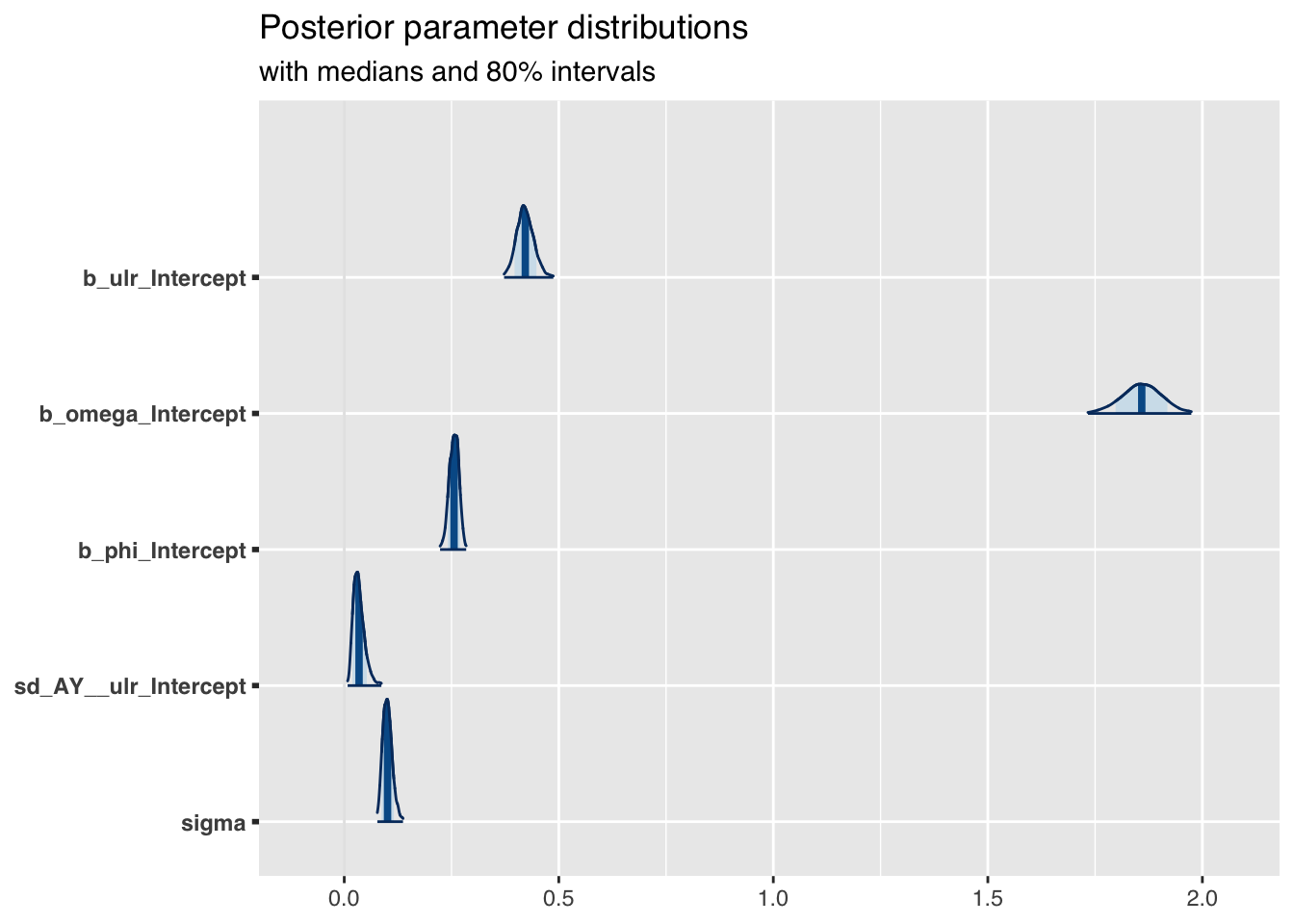
Posterior parameter distributions
The plot of the posterior parameter distributions shows nicely how my priors shrunk:
mcmc_areas(
   as.array(fit_m1),
   pars = c("b_ulr_Intercept", "b_omega_Intercept",
            "b_phi_Intercept",
            "sd_AY__ulr_Intercept", "sigma"),
   prob = 0.8, # 80% intervals
   prob_outer = 0.99, # 99%
   point_est = "mean"
) + ggplot2::labs(
  title = "Posterior parameter distributions",
  subtitle = "with medians and 80% intervals"
)
Posterior predictive distributions
Finally, it is time to plot the posterior predictive distributions:
me_loss_posterior <- marginal_effects(
  fit_m1, conditions = conditions,
  re_formula = NULL, method = "predict"
)
p2 <- plot(me_loss_posterior, ncol = 5, points = TRUE, plot = FALSE)
p2$dev + ggtitle("Posterior predictive distributions")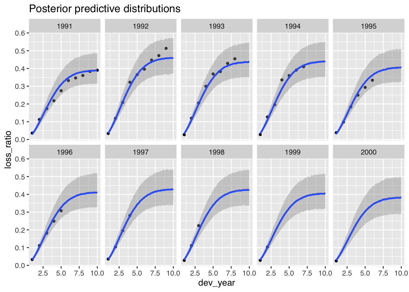
Conclusions
The plot looks good, but the model underestimates the claims development for the 1992 and 1993 accident years.
- Are those years and the data outliers?
- Should the model allow the parameters \(\omega\) and \(\theta\) to vary by year?
- Should I consider a different growth curve family?
Tapping into expert knowledge can be invaluable. However, many domain knowledge experts will not be statisticians and will find it difficult to form an opinion on the ‘Greek’ model or the parameters.
Yet, often experts will have a view on the data generated by the model. Showing them the output of the prior and posterior predictive distributions can be a lot more fruitful.
And as I said earlier, don’t forget they are experts, and hence like/likely to disagree with the non-expert. Use this bias to your advantage!
Update
Jake and I published a new research paper on Hierarchical Compartmental Reserving Models:

Gesmann, M., and Morris, J. “Hierarchical Compartmental Reserving Models.” Casualty Actuarial Society, CAS Research Papers, 19 Aug. 2020, https://www.casact.org/sites/default/files/2021-02/compartmental-reserving-models-gesmannmorris0820.pdf
Session Info
sessionInfo()## R version 4.0.3 (2020-10-10)
## Platform: x86_64-apple-darwin17.0 (64-bit)
## Running under: macOS Big Sur 10.16
##
## Matrix products: default
## BLAS: /Library/Frameworks/R.framework/Versions/4.0/Resources/lib/libRblas.dylib
## LAPACK: /Library/Frameworks/R.framework/Versions/4.0/Resources/lib/libRlapack.dylib
##
## locale:
## [1] en_GB.UTF-8/en_GB.UTF-8/en_GB.UTF-8/C/en_GB.UTF-8/en_GB.UTF-8
##
## attached base packages:
## [1] stats graphics grDevices utils datasets methods base
##
## other attached packages:
## [1] latticeExtra_0.6-29 lattice_0.20-41 data.table_1.13.6
## [4] bayesplot_1.7.2 brms_2.14.4 Rcpp_1.0.5
## [7] rstan_2.21.2 ggplot2_3.3.3 StanHeaders_2.21.0-7
##
## loaded via a namespace (and not attached):
## [1] minqa_1.2.4 colorspace_2.0-0 ellipsis_0.3.1
## [4] ggridges_0.5.2 rsconnect_0.8.16 markdown_1.1
## [7] base64enc_0.1-3 farver_2.0.3 DT_0.16
## [10] fansi_0.4.1 mvtnorm_1.1-1 bridgesampling_1.0-0
## [13] codetools_0.2-18 splines_4.0.3 knitr_1.30
## [16] shinythemes_1.1.2 projpred_2.0.2 jsonlite_1.7.2
## [19] nloptr_1.2.2.2 png_0.1-7 shiny_1.5.0
## [22] compiler_4.0.3 backports_1.2.1 assertthat_0.2.1
## [25] Matrix_1.3-0 fastmap_1.0.1 cli_2.2.0
## [28] later_1.1.0.1 htmltools_0.5.0 prettyunits_1.1.1
## [31] tools_4.0.3 igraph_1.2.6 coda_0.19-4
## [34] gtable_0.3.0 glue_1.4.2 reshape2_1.4.4
## [37] dplyr_1.0.2 V8_3.4.0 vctrs_0.3.6
## [40] nlme_3.1-151 blogdown_0.21 crosstalk_1.1.0.1
## [43] xfun_0.19 stringr_1.4.0 ps_1.5.0
## [46] lme4_1.1-26 mime_0.9 miniUI_0.1.1.1
## [49] lifecycle_0.2.0 gtools_3.8.2 statmod_1.4.35
## [52] MASS_7.3-53 zoo_1.8-8 scales_1.1.1
## [55] colourpicker_1.1.0 promises_1.1.1 Brobdingnag_1.2-6
## [58] parallel_4.0.3 inline_0.3.17 shinystan_2.5.0
## [61] RColorBrewer_1.1-2 gamm4_0.2-6 yaml_2.2.1
## [64] curl_4.3 gridExtra_2.3 loo_2.4.1
## [67] stringi_1.5.3 dygraphs_1.1.1.6 boot_1.3-25
## [70] pkgbuild_1.2.0 rlang_0.4.10 pkgconfig_2.0.3
## [73] matrixStats_0.57.0 evaluate_0.14 purrr_0.3.4
## [76] labeling_0.4.2 rstantools_2.1.1 htmlwidgets_1.5.3
## [79] processx_3.4.5 tidyselect_1.1.0 plyr_1.8.6
## [82] magrittr_2.0.1 bookdown_0.21 R6_2.5.0
## [85] generics_0.1.0 pillar_1.4.7 withr_2.3.0
## [88] mgcv_1.8-33 xts_0.12.1 abind_1.4-5
## [91] tibble_3.0.4 crayon_1.3.4 rmarkdown_2.6
## [94] jpeg_0.1-8.1 grid_4.0.3 callr_3.5.1
## [97] threejs_0.3.3 digest_0.6.27 xtable_1.8-4
## [100] httpuv_1.5.4 RcppParallel_5.0.2 stats4_4.0.3
## [103] munsell_0.5.0 shinyjs_2.0.0References
Citation
For attribution, please cite this work as:Markus Gesmann (Aug 02, 2018) Use domain knowledge to review prior distributions. Retrieved from https://magesblog.com/post/2018-08-02-use-domain-knowledge-to-review-prior-predictive-distributions/
@misc{ 2018-use-domain-knowledge-to-review-prior-distributions,
author = { Markus Gesmann },
title = { Use domain knowledge to review prior distributions },
url = { https://magesblog.com/post/2018-08-02-use-domain-knowledge-to-review-prior-predictive-distributions/ },
year = { 2018 }
updated = { Aug 02, 2018 }
}