PK/PD reserving models
This is a follow-up post on hierarchical compartmental reserving models using PK/PD models. It will show how differential equations can be used with Stan/ brms and how correlation for the same group level terms can be modelled.
PK/ PD is usually short for pharmacokinetic/ pharmacodynamic models, but as Eric Novik of Generable pointed out to me, it could also be short for Payment Kinetics/ Payment Dynamics Models in the insurance context.
In this post I’d like to discuss an extension to Jake Morris’ hierarchical compartmental reserving model, as described in his original paper (Morris (2016)) and my previous post, which allows for a time varying parameter \(k_{er}(t)\) describing the changing rate of earning and reporting and allows for correlation between \(RLR\), the reported loss ratio, and \(RRF\), the reserve robustness factor. A positive correlation would give evidence of a reserving cycle, i.e. in years with higher initial reported loss ratios a higher proportion of reported losses are paid.
I am very grateful for the support Jake Morris and Paul-Christian Bürkner have given me over the last few weeks, answering questions around the model and brms (Bürkner (2017)).
PK/ PD model
First of all let’s take a look at my new set of differential equations, describing the dynamics of exposure (\(EX\)), outstanding (\(OS\)) and paid claims (\(PD\)) over time. I replaced the constant parameter \(k_{er}\) with the linear function \(\beta_{er} \cdot t\).
\[ \begin{aligned} dEX/dt & = -\beta_{er} \cdot t \cdot EX \\ dOS/dt & = \beta_{er} \cdot t \cdot RLR \cdot EX - k_p \cdot OS \\ dPD/dt & = k_{p} \cdot RRF \cdot OS \end{aligned} \]
The dynamical system is no longer autonomous and initially I can’t be bothered to solve it analytically. Hence, I use an ODE solver instead, but I will get back to integrating the differential equations later.
Integrating ODEs with Stan
Fortunately, an ODE solver is part of the Stan language. The following code demonstrates how I can integrate the differential equations in Stan. You will notice that the model section is empty, as all I want to do for now is run the solver.
functions{
  real[] claimsprocess(real t, real [] y, real [] theta,
                       real [] x_r, int[] x_i){
    real dydt[3];
    dydt[1] = - theta[1] * t * y[1];
    dydt[2] = theta[1] * t * theta[3] * y[1] - theta[2] * y[2];
    dydt[3] = theta[2] * theta[4] * y[2];

    return dydt;
  }
}
data {
  real theta[4];
  int N_t;
  real times[N_t];
  real C0[3];
}
parameters{
}
transformed parameters{
  real C[N_t, 3];
  C = integrate_ode_rk45(claimsprocess, C0, 0, times, theta,
                         rep_array(0.0, 0), rep_array(1, 1));
}
model{
}
generated quantities{
  real Exposure[N_t];
  real OS[N_t];
  real Paid[N_t];
  Exposure = C[, 1];
  OS = C[, 2];
  Paid = C[, 3];
}
To run the Stan code I provide as an input a list with the parameters, the number of data points I’d like to generate, the time line and initial starting values. Note also that I have to set the algorithm = "Fixed_param" as I run a deterministic model and for that reason one iteration and one chain are sufficient.
library(rstan)
input_data <- list(
  theta=c(Ber=5, kp=0.5, RLR=0.8, RRF=0.9),
  N_t=100,
  times=seq(from = 0.1, to = 10, length.out = 100),
  C0=c(100, 0, 0))
samples <- sampling(ODEmodel, data=input_data,
                    algorithm = "Fixed_param",
                    iter = 1, chain = 1)
Let’s take a look at the output.
X <- extract(samples)
out <- data.frame(
  Time = input_data$times,
  Exposure = c(X[["Exposure"]]),
  Outstandings = c(X[["OS"]]),
  Paid = c(X[["Paid"]])
)
library(latticeExtra)
xyplot(Exposure + Outstandings + Paid ~ Time,
       data = out, as.table=TRUE, t="l",
       ylab="Amounts ($)", auto.key=list(space="top", columns=3),
       par.settings = theEconomist.theme(with.bg = TRUE, box = "transparent"))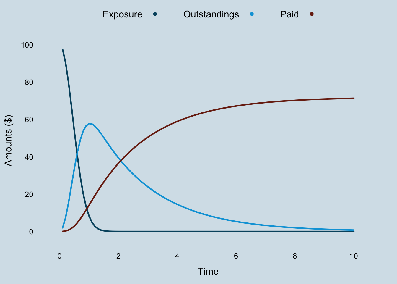
The exposure declines faster and the outstanding curve has a more pronounced peak as a result of replacing \(k_{er}\) with \(\beta_{er} \cdot t\).
Updated model
My updated model is not much different to the one presented in the earlier post, apart from the fact that I allow for the correlation between \(RLR\) and \(RRF\) and the mean function \(\tilde{f}\) is the integral of the ODEs above.
\[ \begin{aligned} y(t) & \sim \mathcal{N}(\tilde{f}(t, \Pi, \beta_{er}, k_p, RLR_{[i]}, RRF_{[i]}), \sigma_{y[\delta]}^2) \\ \begin{pmatrix} RLR_{[i]} \\ RRF_{[i]}\end{pmatrix} & \sim \mathcal{N} \left( \begin{pmatrix} \mu_{RLR} \\ \mu_{RRF} \end{pmatrix}, \begin{pmatrix} \sigma_{RLR}^2 & \rho \ \sigma_{RLR} \sigma_{RRF}\\ \rho \ \sigma_{RLR} \sigma_{RRF} & \sigma_{RRF}^2 \end{pmatrix} \right) \end{aligned} \]
Implementation with brms
Let’s load the data back into R’s memory:
library(data.table)
lossData0 <- fread("https://raw.githubusercontent.com/mages/diesunddas/master/Data/WorkersComp337.csv")
Jake shows in the appendices of his paper how to implement this model in R with the nlmeODE (Tornoe (2012)) package, together with more flexible models in OpenBUGS (Lunn et al. (2000)). However, I will continue with brms and Stan.
Using the ODEs with brms requires a little extra coding, as I have to provide the integration function as an additional input, just like I did above, where I defined them as user defined functions for Stan.
To model the group-level terms (\(RLR\), \(RRF\)) of the same grouping factor (accident year) as correlated I add a unique identifier to the | operator, here I use p (looks similar to \(\rho\)), i.e. ~ 1 + (1 | p | accident_year).
Below is my code for the new updated model. I am using again Gamma distributions as my priors for the parameters and LKJ(2) as a prior for the correlation coefficient.
myFuns <- "
real[] ode_claimsprocess(real t, real [] y,  real [] theta,
                         real [] x_r, int[] x_i){
  real dydt[3];

  dydt[1] = - theta[1] * t * y[1]; // Exposure
  dydt[2] = theta[1] * t * theta[2] * y[1] - theta[3] * y[2]; // OS
  dydt[3] = theta[3] * theta[4] * y[2]; // Paid

  return dydt;
}
real claimsprocess(real t, real premium, real Ber, real kp,
                   real RLR, real RRF, real delta){
  real y0[3];
  real y[1, 3];
  real theta[4];
  theta[1] = Ber;
  theta[2] = RLR;
  theta[3] = kp;
  theta[4] = RRF;
  y0[1] = premium;
  y0[2] = 0;
  y0[3] = 0;
  y = integrate_ode_rk45(ode_claimsprocess,
                        y0, 0, rep_array(t, 1), theta,
                        rep_array(0.0, 0), rep_array(1, 1),
                        0.001, 0.001, 100); // tolerances, steps
      return (y[1, 2] * (1 - delta) + y[1, 3] * delta);
}
"
library(brms)
rstan_options(auto_write = TRUE)
options(mc.cores = parallel::detectCores())
b4 <- brm(
  bf(loss_train ~ claimsprocess(dev, premium, Ber, kp, RLR, RRF, delta),
     RLR ~ 1 + (1 | p | accident_year), # 'p' allow for correlation with RRF
     RRF ~ 1 + (1 | p | accident_year), # 'p' allow for correlation with RLR
     Ber ~ 1,
     kp ~ 1,
     sigma ~ 0 + deltaf, # different sigma for OS and paid
     nl = TRUE),
  stanvars = stanvar(scode = myFuns, block = "functions"),
  data = lossData0[cal <= max(accident_year) & dev > 0],
  family = brmsfamily("gaussian", link_sigma = "log"),
  prior = c(prior(gamma(4, 5), nlpar = "RLR", lb=0),
            prior(gamma(4, 5), nlpar = "RRF", lb=0),
            prior(gamma(12, 3), nlpar = "Ber", lb=0),
            prior(gamma(3, 4), nlpar = "kp", lb=0),
            set_prior("lkj(2)", class = "cor")),
  control = list(adapt_delta = 0.999, max_treedepth=15),
  seed = 1234, iter = 500)
While the original model with the analytical solution ran in about 3 minutes, this code took about 9 hours per chain for 500 samples. Any suggestions how to speed this up will be much appreciated. The frequentist model using nlmeODE runs in seconds.
b4## Warning: There were 235 divergent transitions after warmup. Increasing
## adapt_delta above 0.999 may help. See http://mc-stan.org/misc/
## warnings.html#divergent-transitions-after-warmup## Family: gaussian
## Links: mu = identity; sigma = log
## Formula: loss_train ~ claimsprocess(dev, premium, Ber, kp, RLR, RRF, delta)
## RLR ~ 1 + (1 | p | accident_year)
## RRF ~ 1 + (1 | p | accident_year)
## Ber ~ 1
## kp ~ 1
## sigma ~ 0 + deltaf
## Data: lossData0[cal <= max(accident_year) & dev > 0] (Number of observations: 110)
## Samples: 4 chains, each with iter = 500; warmup = 250; thin = 1;
## total post-warmup samples = 1000
##
## Group-Level Effects:
## ~accident_year (Number of levels: 10)
## Estimate Est.Error l-95% CI u-95% CI Rhat
## sd(RLR_Intercept) 0.18 0.06 0.11 0.32 1.01
## sd(RRF_Intercept) 0.15 0.05 0.09 0.27 1.00
## cor(RLR_Intercept,RRF_Intercept) 0.54 0.24 -0.04 0.88 1.01
## Bulk_ESS Tail_ESS
## sd(RLR_Intercept) 221 281
## sd(RRF_Intercept) 385 534
## cor(RLR_Intercept,RRF_Intercept) 354 392
##
## Population-Level Effects:
## Estimate Est.Error l-95% CI u-95% CI Rhat Bulk_ESS Tail_ESS
## RLR_Intercept 0.86 0.06 0.74 0.99 1.01 176 290
## RRF_Intercept 0.83 0.05 0.73 0.93 1.02 193 414
## Ber_Intercept 5.66 0.32 4.97 6.21 1.01 395 460
## kp_Intercept 0.40 0.01 0.38 0.41 1.00 448 294
## sigma_deltafos -3.61 0.11 -3.81 -3.40 1.00 605 640
## sigma_deltafpaid -4.99 0.11 -5.20 -4.79 1.00 624 507
##
## Samples were drawn using sampling(NUTS). For each parameter, Bulk_ESS
## and Tail_ESS are effective sample size measures, and Rhat is the potential
## scale reduction factor on split chains (at convergence, Rhat = 1).The output above looks very similar to the output of nlmeODE. That’s good, also that Rhat is close to 1 for all parameters. However, there is a warning message of 235 divergent transitions after warm-up, which I will ignore for the time being.
The correlation coefficient \(\rho\) between \(RLR_{[i]}\) and \(RRF_{[i]}\) is estimated as 0.54, but with a wide 95% credible interval from -0.04 to 0.88. Therefore there is moderate evidence of a correlation.
As Jake puts it, a positive correlation between the reported loss ratio and reserve robustness factor parameters by accident year is indicative of a case reserving cycle effect, i.e. more conservative case reserves (low \(RRF_{[i]}\)) in a hard market (low \(RLR_{[i]}\)) to create cushions for the future.
stanplot(b4,
         pars= c("b_RLR_Intercept", "b_RRF_Intercept", "b_Ber_Intercept",
                 "b_kp_Intercept", "b_sigma_deltafos", "b_sigma_deltafpaid",
                 "sd_accident_year__RLR_Intercept",
                 "sd_accident_year__RRF_Intercept",
                 "cor_accident_year__RLR_Intercept__RRF_Intercept"),
         type="dens_overlay")
## Warning: Method 'stanplot' is deprecated. Please use 'mcmc_plot' instead.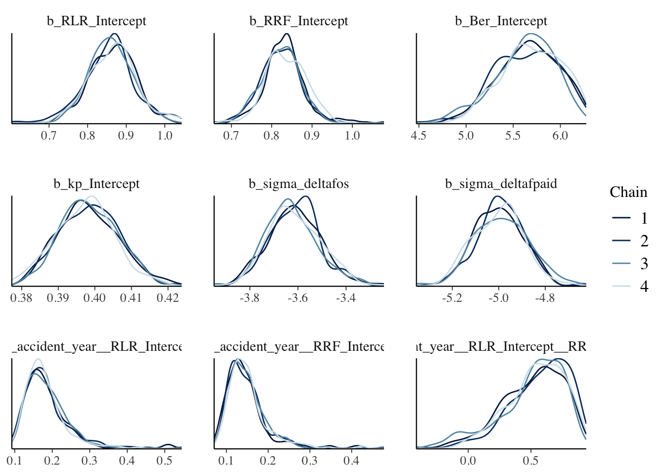
The density plots look OK, all chains seem to have behaved similarly. The last chart in the bottom right shows the distribution of the correlation parameter \(\rho\). Moderate evidence of a correlation might be an understatement. Note also that \(\sigma_{\delta[OS]}\) and \(\sigma_{\delta[PD]}\) are on a log-scale.
Predict future claims developments
To validate my model against the test data set I can use the predict function in brms.
Before I can apply the method I have to expose the Stan functions I wrote above, namely claimsprocess to R.
expose_functions(b4, vectorize = TRUE) # requires brms >= 2.1.0With the claimsprocess function now in the R’s memory I can predict and plot the model in the same way as I did in the previous post.
predClaimsPred <- predict(b4, newdata = lossData0, method="predict")
plotDevBananas(`Q2.5`/premium*100 + `Q97.5`/premium*100 +
                 Estimate/premium*100 + loss_train/premium*100 +
                 loss_test/premium*100 ~
                 dev | factor(accident_year), ylim=c(0, 100),
               data=cbind(lossData0, predClaimsPred)[delta==0],
               main="Outstanding claims developments",
               ylab="Outstanding loss ratio (%)")
plotDevBananas(`Q2.5`/premium*100 + `Q97.5`/premium*100 +
                 Estimate/premium*100 + loss_train/premium*100 +
                 loss_test/premium*100 ~
                 dev | factor(accident_year), ylim=c(0, 120),
               data=cbind(lossData0, predClaimsPred)[delta==1],
               main="Paid claims developments",
               ylab="Paid loss ratio (%)")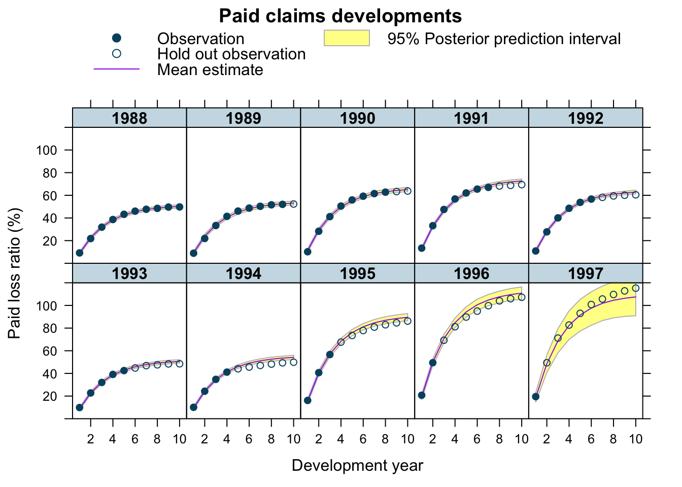
The graphs look very similar to the output from the previous model. Yet, the prediction for 1997 improved significantly, perhaps because of the correlation between RLR and RRF no longer being assumed to be zero. But this model has tested my patience, as I used a remote 2-core machine on Digital Ocean and waited 18 hours for the results.
Analytical solution
The long run time did in the end motivate me to look for an analytical solution of the ODEs, with initial values \(\mbox{EX}(0) = \Pi\) (premium), \(\mbox{OS}(0) = 0\), \(\mbox{PD}(0) = 0\).
According to Wolfram Alpha the analytical solution is:
\[ \begin{aligned} \mbox{EX}(t) & = \Pi \exp \left(-\frac{\beta_{er} t^2}{2} \right) \\ \mbox{OS}(t) & = - \frac{\Pi \cdot RLR}{2 \sqrt{\beta_{er}}} \exp\left(-\frac{\beta_{er} t^2}{2} - k_p t \right) \left[ \sqrt{2 \pi} k_p \mbox{erf}\left(\frac{k_p}{\sqrt{2 \beta_{er}}}\right) \left(-\exp\left(\frac{k_p^2}{2 \beta_{er}} + \frac{\beta_{er} t^2}{2} \right) \right) \right. - \\ & \left. \qquad \sqrt{2 \pi} k_p \exp\left(\frac{k_p^2}{2 \beta_{er}} + \frac{\beta_{er} t^2}{2}\right) \mbox{erf}\left(\frac{\beta_{er} t - k_p}{\sqrt{2 \beta_{er}}}\right) + 2 \sqrt{\beta_{er}} \exp\left(k_p t\right) - 2 \sqrt{\beta_{er}} \exp\left(\frac{\beta_{er} t^2}{2}\right) \right] \\ \mbox{PD}(t) & = \frac{\Pi \cdot RLR \cdot RRF}{2 \sqrt{\beta_{er}}} \exp\left(-k_p t\right) \left[-\sqrt{2 \pi} k_p \exp\left(\frac{k_p^2}{2 \beta_{er}}\right) \mbox{erf}\left(\frac{\beta_{er} t - k_p}{\sqrt{2 \beta_{er}}}\right) \right. + \\ & \left. \qquad \sqrt{2 \pi} k_p \left(-\exp\left(\frac{k^2}{2 \beta_{er}}\right)\right) \mbox{erf}\left(\frac{k}{\sqrt{2 \beta_{er}}} \right) + 2 \sqrt{\beta_{er}} \exp\left(k_p t\right) - 2 \sqrt{\beta_{er}} \right] \end{aligned} \]
Now I can write down \(\tilde{f}(t)\) in a closed-form: \[ \tilde{f}(t, \delta,\dots) = (1 - \delta) \cdot \mbox{OS}(t, \dots) + \delta \cdot \mbox{PD}(t, \dots) \]
The error function is part of the Stan language (not directly in R, although it is just erf <- function(x) 2 * pnorm(x * sqrt(2)) - 1). Thus, I create a Stan function for the analytical claims process again and feed this into brm.
library(brms)
library(rstan)
rstan_options(auto_write = TRUE)
options(mc.cores = parallel::detectCores())

myFun <- "
real anaclaimsprocess(real t, real premium, real Ber, real kp,
                      real RLR, real RRF, real delta){

 real os;
 real paid;

 os = -(RLR * exp(-(Ber * t^2)/2.0 - kp * t) *
          (sqrt(2.0 * pi()) * kp * erf(kp/(sqrt(2.0) * sqrt(Ber))) *
             (-exp(kp^2/(2.0 * Ber) + (Ber * t^2)/2.0)) -
             sqrt(2.0 * pi()) * kp * exp(kp^2/(2.0 * Ber) + (Ber *t^2)/2.0) *
             erf((Ber*t - kp)/(sqrt(2.0) * sqrt(Ber))) +
             2.0 * sqrt(Ber) * exp(kp * t) - 2.0 * sqrt(Ber) *
             exp((Ber*t^2)/2.0)))/(2.0 * sqrt(Ber));
 paid = (RLR * RRF * exp(-kp * t) *
           (-sqrt(2.0 * pi()) * kp * exp(kp^2/(2.0 * Ber)) *
              erf((Ber*t - kp)/(sqrt(2.0) * sqrt(Ber))) +
              sqrt(2.0 * pi()) * kp * (-exp(kp^2/(2.0 * Ber))) *
              erf(kp/(sqrt(2.0) * sqrt(Ber))) + 2.0 * sqrt(Ber) * exp(kp * t) -
              2.0 * sqrt(Ber)))/(2.0 * sqrt(Ber));

 return (premium * (os * (1 - delta) + paid * delta));
}
"

b5 <- brm(bf(loss_train ~ anaclaimsprocess(dev, premium, Ber, kp,
                                           RLR, RRF, delta),
             RLR ~ 1 + (1 | p | accident_year),
             RRF ~ 1 + (1 | p | accident_year),
             Ber ~ 1,
             kp ~ 1,
             sigma ~ 0 + deltaf,
             nl = TRUE),
          stanvars = stanvar(scode = myFun, block = "functions"),
          data = lossData0[cal <= max(accident_year)],
          family = brmsfamily("gaussian", link_sigma = "log"),
          prior = c(prior(gamma(4, 5), nlpar = "RLR", lb=0),
                    prior(gamma(4, 5), nlpar = "RRF", lb=0),
                    prior(gamma(12, 3), nlpar = "Ber", lb=0),
                    prior(gamma(3, 4), nlpar = "kp", lb=0),
                    set_prior("lkj(2)", class = "cor")),
          control = list(adapt_delta = 0.999, max_treedepth=15),
          file="pkpdmodel_b5.rds",
          seed = 1234, iter = 1000)
Wonderful, the code ran in about 5 minutes, with twice the number of samples and without any warnings messages. Let’s take a look at the output:
b5## Family: gaussian
## Links: mu = identity; sigma = log
## Formula: loss_train ~ anaclaimsprocess(dev, premium, Ber, kp, RLR, RRF, delta)
## RLR ~ 1 + (1 | p | accident_year)
## RRF ~ 1 + (1 | p | accident_year)
## Ber ~ 1
## kp ~ 1
## sigma ~ 0 + deltaf
## Data: lossData0[cal <= max(accident_year)] (Number of observations: 110)
## Samples: 4 chains, each with iter = 1000; warmup = 500; thin = 1;
## total post-warmup samples = 2000
##
## Group-Level Effects:
## ~accident_year (Number of levels: 10)
## Estimate Est.Error l-95% CI u-95% CI Rhat
## sd(RLR_Intercept) 0.18 0.05 0.11 0.32 1.00
## sd(RRF_Intercept) 0.15 0.05 0.09 0.28 1.00
## cor(RLR_Intercept,RRF_Intercept) 0.52 0.25 -0.11 0.88 1.00
## Bulk_ESS Tail_ESS
## sd(RLR_Intercept) 680 877
## sd(RRF_Intercept) 671 1342
## cor(RLR_Intercept,RRF_Intercept) 822 998
##
## Population-Level Effects:
## Estimate Est.Error l-95% CI u-95% CI Rhat Bulk_ESS Tail_ESS
## RLR_Intercept 0.86 0.06 0.73 0.99 1.01 586 519
## RRF_Intercept 0.83 0.05 0.72 0.93 1.01 614 518
## Ber_Intercept 5.69 0.35 5.07 6.40 1.00 1860 1470
## kp_Intercept 0.40 0.01 0.38 0.41 1.00 1869 1733
## sigma_deltafos -3.61 0.11 -3.81 -3.39 1.00 1945 1531
## sigma_deltafpaid -4.99 0.11 -5.20 -4.77 1.00 1818 1183
##
## Samples were drawn using sampling(NUTS). For each parameter, Bulk_ESS
## and Tail_ESS are effective sample size measures, and Rhat is the potential
## scale reduction factor on split chains (at convergence, Rhat = 1).Perfect, the estimates are very much the same as from the ODE model and the plots haven’t changed much either.
mcmc_plot(b5,
         pars= c("b_RLR_Intercept", "b_RRF_Intercept", "b_Ber_Intercept",
                 "b_kp_Intercept", "b_sigma_deltafos", "b_sigma_deltafpaid",
                 "sd_accident_year__RLR_Intercept",
                 "sd_accident_year__RRF_Intercept",
                 "cor_accident_year__RLR_Intercept__RRF_Intercept"),
         type="dens_overlay")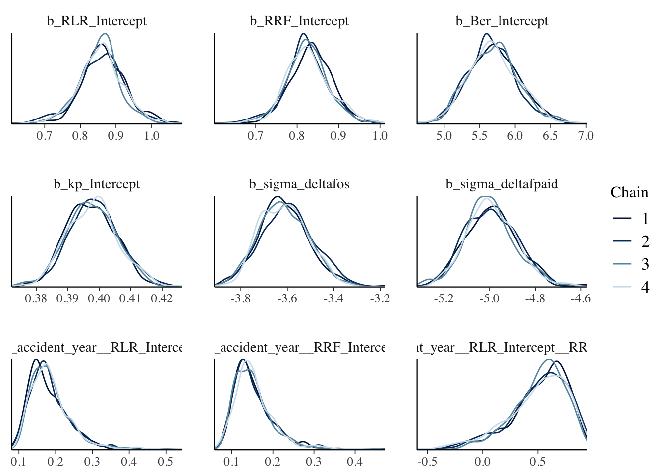
The density plots look smoother and more consistent across chains with twice the number of samples compared to the previous model.
expose_functions(b5, vectorize = TRUE) # requires brms >= 2.1.0predClaimsPred2 <- predict(b5, newdata = lossData0, method="predict")
plotDevBananas(`Q2.5`/premium*100 + `Q97.5`/premium*100 +
Estimate/premium*100 + loss_train/premium*100 +
loss_test/premium*100 ~
dev | factor(accident_year), ylim=c(0, 100),
data=cbind(lossData0, predClaimsPred2)[delta==0],
main="Outstanding claims developments",
ylab="Outstanding loss ratio (%)")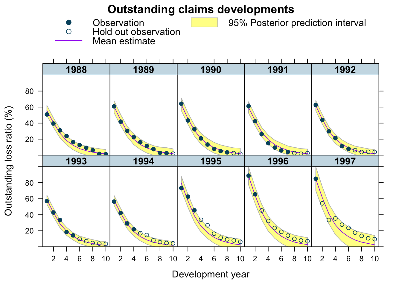
plotDevBananas(`Q2.5`/premium*100 + `Q97.5`/premium*100 +
                 Estimate/premium*100 + loss_train/premium*100 +
                 loss_test/premium*100 ~
                 dev | factor(accident_year), ylim=c(0, 120),
               data=cbind(lossData0, predClaimsPred2)[delta==1],
               main="Paid claims developments",
               ylab="Paid loss ratio (%)")
I am much happier now. The model runs in an acceptable time, allowing me to play around with my assumptions further. I have yet to understand why the integration routine in Stan took so long.
Update
Jake and I published a new research paper on Hierarchical Compartmental Reserving Models:
Gesmann, M., and Morris, J. “Hierarchical Compartmental Reserving Models.” Casualty Actuarial Society, CAS Research Papers, 19 Aug. 2020, https://www.casact.org/sites/default/files/2021-02/compartmental-reserving-models-gesmannmorris0820.pdf
Session Info
sessionInfo()## R version 4.0.3 (2020-10-10)
## Platform: x86_64-apple-darwin17.0 (64-bit)
## Running under: macOS Big Sur 10.16
##
## Matrix products: default
## BLAS: /Library/Frameworks/R.framework/Versions/4.0/Resources/lib/libRblas.dylib
## LAPACK: /Library/Frameworks/R.framework/Versions/4.0/Resources/lib/libRlapack.dylib
##
## locale:
## [1] en_GB.UTF-8/en_GB.UTF-8/en_GB.UTF-8/C/en_GB.UTF-8/en_GB.UTF-8
##
## attached base packages:
## [1] stats graphics grDevices utils datasets methods base
##
## other attached packages:
## [1] brms_2.14.4 Rcpp_1.0.5 data.table_1.13.6
## [4] latticeExtra_0.6-29 lattice_0.20-41 rstan_2.21.2
## [7] ggplot2_3.3.3 StanHeaders_2.21.0-7
##
## loaded via a namespace (and not attached):
## [1] minqa_1.2.4 colorspace_2.0-0 RcppEigen_0.3.3.9.1
## [4] ellipsis_0.3.1 ggridges_0.5.2 rsconnect_0.8.16
## [7] markdown_1.1 base64enc_0.1-3 farver_2.0.3
## [10] DT_0.16 fansi_0.4.1 mvtnorm_1.1-1
## [13] bridgesampling_1.0-0 codetools_0.2-18 splines_4.0.3
## [16] knitr_1.30 shinythemes_1.1.2 bayesplot_1.7.2
## [19] projpred_2.0.2 jsonlite_1.7.2 nloptr_1.2.2.2
## [22] png_0.1-7 shiny_1.5.0 compiler_4.0.3
## [25] backports_1.2.1 assertthat_0.2.1 Matrix_1.3-0
## [28] fastmap_1.0.1 cli_2.2.0 later_1.1.0.1
## [31] htmltools_0.5.0 prettyunits_1.1.1 tools_4.0.3
## [34] igraph_1.2.6 coda_0.19-4 gtable_0.3.0
## [37] glue_1.4.2 reshape2_1.4.4 dplyr_1.0.2
## [40] V8_3.4.0 vctrs_0.3.6 nlme_3.1-151
## [43] blogdown_0.21 crosstalk_1.1.0.1 xfun_0.19
## [46] stringr_1.4.0 ps_1.5.0 lme4_1.1-26
## [49] mime_0.9 miniUI_0.1.1.1 lifecycle_0.2.0
## [52] gtools_3.8.2 statmod_1.4.35 MASS_7.3-53
## [55] zoo_1.8-8 scales_1.1.1 colourpicker_1.1.0
## [58] promises_1.1.1 Brobdingnag_1.2-6 parallel_4.0.3
## [61] inline_0.3.17 shinystan_2.5.0 RColorBrewer_1.1-2
## [64] gamm4_0.2-6 yaml_2.2.1 curl_4.3
## [67] gridExtra_2.3 loo_2.4.1 stringi_1.5.3
## [70] dygraphs_1.1.1.6 boot_1.3-25 pkgbuild_1.2.0
## [73] rlang_0.4.10 pkgconfig_2.0.3 matrixStats_0.57.0
## [76] BH_1.72.0-3 evaluate_0.14 purrr_0.3.4
## [79] rstantools_2.1.1 htmlwidgets_1.5.3 labeling_0.4.2
## [82] processx_3.4.5 tidyselect_1.1.0 plyr_1.8.6
## [85] magrittr_2.0.1 bookdown_0.21 R6_2.5.0
## [88] generics_0.1.0 pillar_1.4.7 withr_2.3.0
## [91] mgcv_1.8-33 xts_0.12.1 abind_1.4-5
## [94] tibble_3.0.4 crayon_1.3.4 rmarkdown_2.6
## [97] jpeg_0.1-8.1 grid_4.0.3 callr_3.5.1
## [100] threejs_0.3.3 digest_0.6.27 xtable_1.8-4
## [103] httpuv_1.5.4 RcppParallel_5.0.2 stats4_4.0.3
## [106] munsell_0.5.0 shinyjs_2.0.0References
Citation
For attribution, please cite this work as:Markus Gesmann (Jan 30, 2018) PK/PD reserving models. Retrieved from https://magesblog.com/post/2018-01-30-pkpd-reserving-models/
@misc{ 2018-pk/pd-reserving-models,
author = { Markus Gesmann },
title = { PK/PD reserving models },
url = { https://magesblog.com/post/2018-01-30-pkpd-reserving-models/ },
year = { 2018 }
updated = { Jan 30, 2018 }
}
