Hierarchical Loss Reserving with Stan
I continue with the growth curve model for loss reserving from last week’s post. Today, following the ideas of James Guszcza [2] I will add an hierarchical component to the model, by treating the ultimate loss cost of an accident year as a random effect. Initially, I will use the nlme R package, just as James did in his paper, and then move on to Stan/RStan [6], which will allow me to estimate the full distribution of future claims payments.
The growth curve describes the proportion of claims paid up to a given development period compared to the ultimate claims cost at the end of time, hence often called development pattern. Cumulative distribution functions are often considered, as they increase monotonously from 0 to 100%. Multiplying the development pattern with the expected ultimate loss cost gives me then the expected cumulative paid to date value.
However, what I’d like to do is the opposite, I know the cumulative claims position to date and wish to estimate the ultimate claims cost instead. If the claims process is fairly stable over the years and say, once a claim has been notified the payment process is quite similar from year to year and claim to claim, then a growth curve model is not unreasonable. Yet, the number and the size of the yearly claims will be random, e.g. if a windstorm, fire, etc occurs or not. Hence, a random effect for the ultimate loss cost across accident years sounds very convincing to me.
Here is James’ model as described in [2]:
\[ \begin{aligned} CL_{AY, dev} & \sim \mathcal{N}(\mu_{AY, dev}, \sigma^2_{dev}) \\ \mu_{AY,dev} & = Ult_{AY} \cdot G(dev|\omega, \theta)\\ \sigma_{dev} & = \sigma \sqrt{\mu_{dev}}\\ Ult_{AY} & \sim \mathcal{N}(\mu_{ult}, \sigma^2_{ult})\\ G(dev|\omega, \theta) & = 1 - \exp\left(-\left(\frac{dev}{\theta}\right)^\omega\right) \end{aligned} \]
The cumulative losses \(CL_{AY, dev}\) for a given accident year \(AY\) and development period \(dev\) follow a Normal distribution with parameters \(\mu_{AY, dev}\) and \(\sigma_{dev}\).
The mean itself is modelled as the product of an accident year specific ultimate loss cost \(Ult_{AY}\) and a development period specific parametric growth curve \(G(dev | \omega, \theta)\). The variance is believed to increase in proportion with the mean. Finally, the ultimate loss cost is modelled with a Normal distribution as well.
Assuming a Gaussian distribution of losses doesn’t sound quite intuitive to me, as loss are often skewed to the right, but I shall continue with this assumption here to make a comparison with [2] possible.
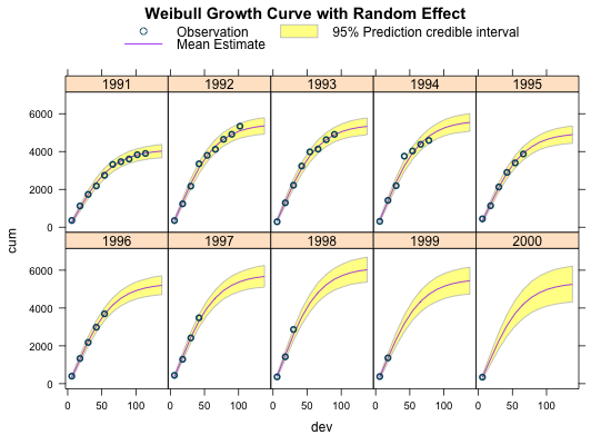
Using the example data set given in the paper I can reproduce the result in R withnlme:
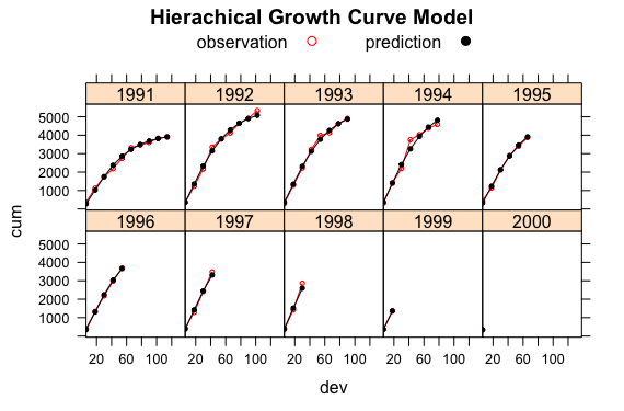
The fit looks pretty good, with only 5 parameters. See James’ paper for a more detailed discussion.
Let’s move this model into Stan. Here is my attempt, which builds on last week’s pooled model. With the generated quantities code block I go beyond the scope of the original paper, as I try to estimate the full posterior predictive distribution as well.The ‘trick’ is the line mu[i] <- ult[origin[i]] * weibull_cdf(dev[i], omega, theta); where I have an accident year (here labelled origin) specific ultimate loss.
The notation ult[origin[i]] illustrates the hierarchical nature in Stan’s language nicely.
The estimated parameters look very similar to the nlme output above.
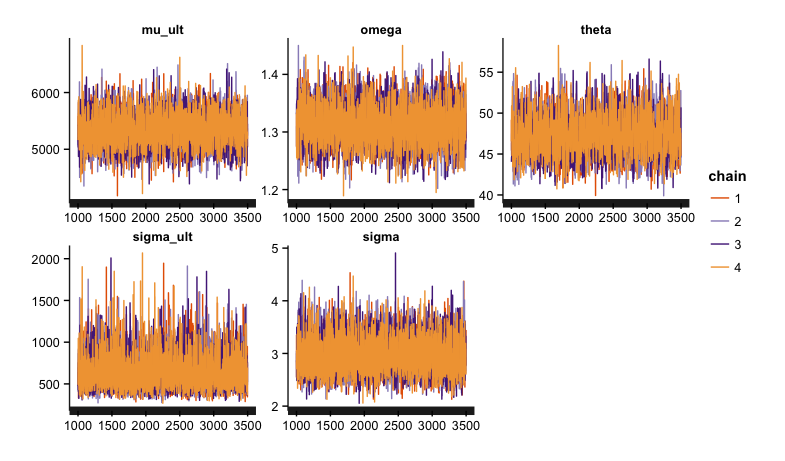
This looks all not too bad. The trace plots don’t show any particular patterns, apart from \(\sigma_{ult}\), which shows a little skewness.
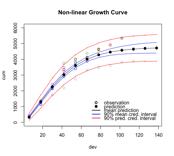
Thegenerated quantities code block in Stan allows me to get also the predictive distribution beyond the current data range. Here I forecast claims up to development year 12 and plot the predictions, including the 95% credibility interval of the posterior predictive distribution with the observations.
Conclusions
The Bayesian approach sounds to me a lot more natural than many classical techniques around the chain-ladder methods. Thanks to Stan, I can get the full posterior distributions on both, the parameters and predictive distribution. I find communicating credibility intervals much easier than talking about the parameter, process and mean squared error.
James Guszcza contributed to a follow-up paper with Y. Zhank and V. Dukic [3] that extends the model described in [2]. It deals with skewness in loss data sets and the autoregressive nature of the errors in a cumulative time series.
Frank Schmid offers a more complex Bayesian analysis of claims reserving in [4], while Jake Morris highlights the similarities between a compartmental model used in drug research and loss reserving [5].
Finally, Glenn Meyers published a monograph on Stochastic Loss Reserving Using Bayesian MCMC Models earlier this year [7] that is worth taking a look at.
Update
Jake Morris and I published a new research paper on Hierarchical Compartmental Reserving Models:
Gesmann, M., and Morris, J. “Hierarchical Compartmental Reserving Models.” Casualty Actuarial Society, CAS Research Papers, 19 Aug. 2020, https://www.casact.org/sites/default/files/2021-02/compartmental-reserving-models-gesmannmorris0820.pdf
References
[1] David R. Clark. LDF Curve-Fitting and Stochastic Reserving: A Maximum Likelihood Approach. Casualty Actuarial Society, 2003. CAS Fall Forum.
[2] James Guszcza. Hierarchical Growth Curve Models for Loss Reserving, 2008, CAS Fall Forum, pp. 146–173.
[3] Y. Zhang, V. Dukic, and James Guszcza. A Bayesian non-linear model for forecasting insurance loss payments. 2012. Journal of the Royal Statistical Society: Series A (Statistics in Society), 175: 637–656. doi: 10.1111/j.1467-985X.2011.01002.x
[4] Frank A. Schmid. Robust Loss Development Using MCMC. Available at SSRN. See also http://lossdev.r-forge.r-project.org/
[5] Jake Morris. Compartmental reserving in R. 2015. R in Insurance Conference.
[6] Stan Development Team. Stan: A C++ Library for Probability and Sampling, Version 2.8.0. 2015. http://mc-stan.org/.
[7] Glenn Meyers. Stochastic Loss Reserving Using Bayesian MCMC Models. Issue 1 of CAS Monograph Series. 2015.Session Info
R version 3.2.2 (2015-08-14)
Platform: x86_64-apple-darwin13.4.0 (64-bit)
Running under: OS X 10.11.1 (El Capitan)

locale:
[1] en_GB.UTF-8/en_GB.UTF-8/en_GB.UTF-8/C/en_GB.UTF-8/en_GB.UTF-8

attached base packages:
[1] stats  graphics  grDevices utils datasets  methods   base

other attached packages:
[1] ChainLadder_0.2.3 rstan_2.8.0   ggplot2_1.0.1  Rcpp_0.12.1
[5] lattice_0.20-33

loaded via a namespace (and not attached):
 [1] nloptr_1.0.4       plyr_1.8.3         tools_3.2.2
 [4] digest_0.6.8       lme4_1.1-10        statmod_1.4.21
 [7] gtable_0.1.2       nlme_3.1-122       mgcv_1.8-8
[10] Matrix_1.2-2       parallel_3.2.2     biglm_0.9-1
[13] SparseM_1.7        proto_0.3-10       coda_0.18-1
[16] gridExtra_2.0.0    stringr_1.0.0      MatrixModels_0.4-1
[19] lmtest_0.9-34      stats4_3.2.2       grid_3.2.2
[22] nnet_7.3-11        tweedie_2.2.1      inline_0.3.14
[25] cplm_0.7-4         minqa_1.2.4        actuar_1.1-10
[28] reshape2_1.4.1     car_2.1-0          magrittr_1.5
[31] scales_0.3.0       codetools_0.2-14   MASS_7.3-44
[34] splines_3.2.2      rsconnect_0.3.79   systemfit_1.1-18
[37] pbkrtest_0.4-2     colorspace_1.2-6   quantreg_5.19
[40] labeling_0.3       sandwich_2.3-4     stringi_1.0-1
[43] munsell_0.4.2      zoo_1.7-12
Citation
For attribution, please cite this work as:Markus Gesmann (Nov 10, 2015) Hierarchical Loss Reserving with Stan. Retrieved from https://magesblog.com/post/2015-11-10-hierarchical-loss-reserving-with-stan/
@misc{ 2015-hierarchical-loss-reserving-with-stan,
author = { Markus Gesmann },
title = { Hierarchical Loss Reserving with Stan },
url = { https://magesblog.com/post/2015-11-10-hierarchical-loss-reserving-with-stan/ },
year = { 2015 }
updated = { Nov 10, 2015 }
}