Reserving based on log-incremental payments in R, part II
Following on from last week’s post I will continue to go through the paper Regression models based on log-incremental payments by Stavros Christofides [1]. In the previous post I introduced the model from the first 15 pages up to section F. Today I will progress with sections G to K which illustrate the model with a more realistic incremental claims payments triangle from a UK Motor Non-Comprehensive account:
# Page D5.17
tri <- t(matrix(
  c(3511, 3215, 2266, 1712, 1059, 587, 340,
    4001, 3702, 2278, 1180,  956, 629,  NA,
    4355, 3932, 1946, 1522, 1238,  NA,  NA,
    4295, 3455, 2023, 1320,   NA,  NA,  NA,
    4150, 3747, 2320,   NA,   NA,  NA,  NA,
    5102, 4548,   NA,   NA,   NA,  NA,  NA,
    6283,   NA,   NA,   NA,   NA,  NA,  NA), nc=7))
The rows show origin period data, e.g. accident years, underwriting years or years of account and the columns present the development periods or lags. The triangle appears to be fairly well behaved. The last two years in rows 6 and 7 appear to be slightly higher than rows 2 to 5 and the values in row 1 are lower in comparison to the later years. The last payment of £1,238 in the third row stands out a bit as well.
Before I plot the data, I will transform the triangle into a data frame and add extra columns:
m <- dim(tri)[1]; n <- dim(tri)[2]
dat <- data.frame(
  origin=rep(0:(m-1), n),
  dev=rep(0:(n-1), each=m),
  value=as.vector(tri))

## Add dimensions as factors
dat <- with(dat, data.frame(origin, dev, cal=origin+dev,
                            value, logvalue=log(value),
                            originf=factor(origin),
                            devf=as.factor(dev),
                            calf=as.factor(origin+dev)))
I am particularly interested in the decay of claims payments in the development year direction for each origin year on the original and log-scale. The interaction.plot of the stats package does an excellent job for this:
op <- par(mfrow=c(2,1), mar=c(4,4,2,2))
with(dat, interaction.plot(x.factor=dev, trace.factor=origin,
                           response=value))
points(dat$devf, dat$value, pch=16, cex=0.5)
with(dat, interaction.plot(x.factor=dev, trace.factor=origin,
                           response=logvalue))
points(dat$devf, dat$logvalue, pch=16, cex=0.5)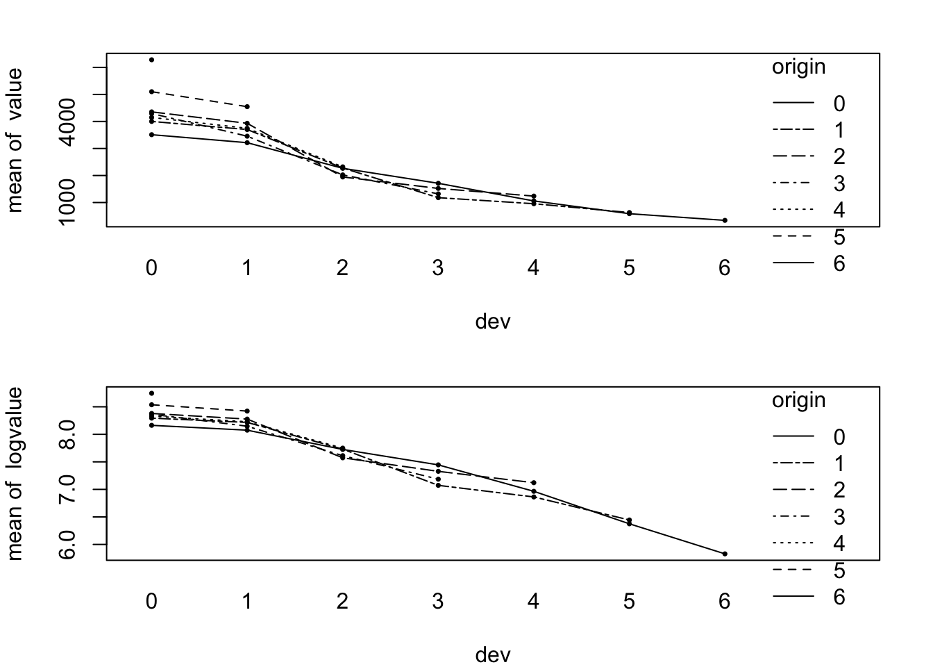
par(op)Indeed the origin years 1 to 4 (rows 2 to 5) look quite similar and the decay of claims in development year direction appears to be linear on a log-scale from development year 1 onwards.
Based on those observations Christofides suggests two models; the first one will have a unique level for each origin year and a unique level for the zero development period. The parameters for development periods 1 to 6 are assumed to follow a linear relationship with the same slope:
\[ \begin{aligned} \log{(P_{ij})} & = Y_{ij} = a_i + d_j + \epsilon_{ij} \mbox{ for } i,j \mbox{ from } 0 \mbox{ to } 6 \\ & \mbox{where } d_0 = d, d_j = s \cdot j\mbox{ for } j > 0 \end{aligned} \]
and \(\epsilon_{ij} \sim N(0, \sigma^2)\). The second model will be a reduced version of the above with only two levels for the origin years 5 and 6. Hence, I add four more columns to my data frame:
dat <- with(dat,
            data.frame(dat,
                       a6 = ifelse(origin == 6, 1, 0),
                       a5 = ifelse(origin == 5, 1, 0),
                       d = ifelse(dev < 1, 1, 0),
                       s = ifelse(dev < 1, 0, dev)))

dat <- dat[order(dat$origin),] # to have similar output as in the paper
As in the earlier section of the paper and my previous post, I start with a model using all levels of the origin factor:
# Page D5.20/21
summary(Fit1 <- lm(logvalue ~ 0 + originf + d + s, data=na.omit(dat)))
##
## Call:
## lm(formula = logvalue ~ 0 + originf + d + s, data = na.omit(dat))
##
## Residuals:
## Min 1Q Median 3Q Max
## -0.22142 -0.03973 0.01116 0.03289 0.19622
##
## Coefficients:
## Estimate Std. Error t value Pr(>|t|)
## originf0 8.57284 0.07569 113.262 < 2e-16 ***
## originf1 8.57379 0.07152 119.884 < 2e-16 ***
## originf2 8.66487 0.06936 124.923 < 2e-16 ***
## originf3 8.55412 0.07022 121.814 < 2e-16 ***
## originf4 8.63666 0.07587 113.841 < 2e-16 ***
## originf5 8.84550 0.09059 97.646 < 2e-16 ***
## originf6 9.04182 0.13368 67.638 < 2e-16 ***
## d -0.29622 0.06990 -4.238 0.000445 ***
## s -0.43496 0.01849 -23.526 1.63e-15 ***
## ---
## Signif. codes: 0 '***' 0.001 '**' 0.01 '*' 0.05 '.' 0.1 ' ' 1
##
## Residual standard error: 0.1139 on 19 degrees of freedom
## Multiple R-squared: 0.9999, Adjusted R-squared: 0.9998
## F-statistic: 1.428e+04 on 9 and 19 DF, p-value: < 2.2e-16Clearly all origin levels are significantly different from zero, yet most of them are actually quite similar. The tests in the above output don’t make much sense as they test the various intercepts against zero. That’s easy to fix, I take out the first term ‘0 +’, which forced lm to fit individual intercepts. The next model makes much more sense:
# Page D5.21/22
summary(Fit2 <- lm(logvalue ~ originf + d + s, data=na.omit(dat)))
##
## Call:
## lm(formula = logvalue ~ originf + d + s, data = na.omit(dat))
##
## Residuals:
## Min 1Q Median 3Q Max
## -0.22142 -0.03973 0.01116 0.03289 0.19622
##
## Coefficients:
## Estimate Std. Error t value Pr(>|t|)
## (Intercept) 8.5728353 0.0756903 113.262 < 2e-16 ***
## originf1 0.0009565 0.0639346 0.015 0.988220
## originf2 0.0920366 0.0686753 1.340 0.195997
## originf3 -0.0187149 0.0752609 -0.249 0.806287
## originf4 0.0638284 0.0843021 0.757 0.458254
## originf5 0.2726676 0.0982451 2.775 0.012052 *
## originf6 0.4689829 0.1315930 3.564 0.002072 **
## d -0.2962154 0.0699026 -4.238 0.000445 ***
## s -0.4349597 0.0184885 -23.526 1.63e-15 ***
## ---
## Signif. codes: 0 '***' 0.001 '**' 0.01 '*' 0.05 '.' 0.1 ' ' 1
##
## Residual standard error: 0.1139 on 19 degrees of freedom
## Multiple R-squared: 0.9832, Adjusted R-squared: 0.9762
## F-statistic: 139.1 on 8 and 19 DF, p-value: 3.287e-15Following Christofides I reduce the model, assuming a constant intercept (or constant claims in development period 0) for the origin years 0 to 4 and separate ones for the the origin years 5 and 6:
# Page D5.23
summary(Fit3 <- lm(logvalue ~ a5 + a6 + d + s, data=na.omit(dat)))
##
## Call:
## lm(formula = logvalue ~ a5 + a6 + d + s, data = na.omit(dat))
##
## Residuals:
## Min 1Q Median 3Q Max
## -0.21567 -0.04910 0.00654 0.05137 0.27198
##
## Coefficients:
## Estimate Std. Error t value Pr(>|t|)
## (Intercept) 8.60795 0.05150 167.142 < 2e-16 ***
## a5 0.24353 0.08517 2.859 0.008870 **
## a6 0.44111 0.12170 3.625 0.001421 **
## d -0.30345 0.06779 -4.476 0.000172 ***
## s -0.43967 0.01666 -26.390 < 2e-16 ***
## ---
## Signif. codes: 0 '***' 0.001 '**' 0.01 '*' 0.05 '.' 0.1 ' ' 1
##
## Residual standard error: 0.1119 on 23 degrees of freedom
## Multiple R-squared: 0.9804, Adjusted R-squared: 0.977
## F-statistic: 287.7 on 4 and 23 DF, p-value: < 2.2e-16Wonderful, all coefficients appear to be significant and I am left with a model of only five parameters. Next I look at the residual plots:
# Resdiual plots
op <- par(mfrow=c(2,2), mar=c(4,4,2,2))
attach(model.frame(Fit3))
with(na.omit(dat),
     plot.default(rstandard(Fit3) ~ origin,
                  main="Residuals vs. origin years"))
abline(h=0, lty=2)

with(na.omit(dat),
     plot.default(rstandard(Fit3) ~ dev,
                  main="Residuals vs. dev. years"))
abline(h=0, lty=2)
with(na.omit(dat),
     plot.default(rstandard(Fit3) ~ cal,
                  main="Residuals vs. payments years"))
abline(h=0, lty=2)
plot.default(rstandard(Fit3) ~ logvalue,
             main="Residuals vs. fitted")
abline(h=0, lty=2)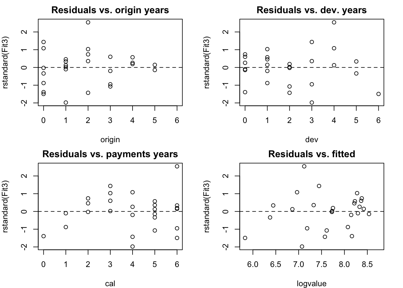
detach(model.frame(Fit3))
par(op)
The residual plots look quite well behaved. The last payment in year 2 does appear to be a bit of an outlier and also the pattern in the payment or calendar year direction gives an indication of potential claims inflation which should be investigated further.
Following the paper and for the purpose of this post I want to focus on deriving estimators for the payments in future years and their standard errors. I did most of the leg work last week, so I here bring the various calculations for the forecast and error estimation together into a new function:
log.incr.predict <- function(
    model, # lm output
    newdata, # same argument as in predict
    origin.var = "origin", # name of the origin column in newdata
    dev.var = "dev" # name of the dev column in newdata
){
  origin <- newdata[[origin.var]]
  dev <- newdata[[dev.var]]

  Pred <- predict(model, newdata=newdata, se.fit=TRUE)

  Y <- Pred$fit
  VarY <- Pred$se.fit^2 + Pred$residual.scale^2
  P <- exp(Y + VarY/2)
  VarP <-  exp(2*Y + VarY)*(exp(VarY)-1)
  seP <- sqrt(VarP)

  ## Recreate formula to derive the model.frame and future design matrix
  model.formula <- as.formula(paste("~", as.character(formula(model)[3])))
  ## See also package formula.tool

  mframe <- model.frame(model.formula, data=newdata)
  fdm <- model.matrix(model.formula, data=newdata)
  varcovar <- fdm %*% vcov(model) %*% t(fdm)

  sigma <- summary(model)$sigma
  dsigma2 <- diag(sigma^2, nrow = dim(varcovar)[1])
  OverallVar <- t(P) %*% (exp(dsigma2 + varcovar) - 1) %*% P
  Total.SE <- sqrt(OverallVar)
  Total.Reserve <- sum(P)

  # Prepare output
  Incr <- data.frame(origin, dev, Y, VarY, P, seP, CV=seP/P)
  out <- list(
    Forecast = Incr[order(newdata[[origin.var]]),],
    Totals = data.frame(Total.Reserve,
                        Total.SE=Total.SE,
                        CV=Total.SE/Total.Reserve)
  )
  return(out)
}
With the above function it is straightforward to carry out the prediction of future claims payments and standard errors. As a bonus I can estimate claims payments beyond the available data, as my models assume an exponential decay. Here I will assume in line with Christofides that claims payments will stop 6 years after the latest available development data:
tail.years <- 6
# Create a data frame for the future periods
fdat <- data.frame(
  origin = rep(0:(m-1), n+tail.years),
  dev = rep(0:(n+tail.years-1), each=m)
)
fdat$cal <- with(fdat, origin + dev)

fdat <- with(fdat,
             data.frame(fdat,
                        originf = factor(origin),
                        a6 = ifelse(origin == 6, 1, 0),
                        a5 = ifelse(origin == 5, 1, 0),
                        d = ifelse(dev < 1, 1, 0),
                        s = ifelse(dev < 1, 0, dev)))
So, here are the results for my two models:
FM2 <- log.incr.predict(Fit2, subset(fdat, cal>6))
FM2 # Page D5.32/33
## $Forecast
## origin dev Y VarY P seP CV
## 50 0 7 5.528118 0.01947679 254.13254 35.639951 0.1402416
## 57 0 8 5.093158 0.02232053 164.73171 24.748983 0.1502381
## 64 0 9 4.658198 0.02584791 106.81754 17.284935 0.1618174
## 71 0 10 4.223239 0.03005895 69.28774 12.103614 0.1746862
## 78 0 11 3.788279 0.03495363 44.95921 8.479513 0.1886046
## 85 0 12 3.353319 0.04053196 29.18296 5.935315 0.2033829
## 44 1 6 5.964034 0.01852071 392.79744 53.704591 0.1367234
## 51 1 7 5.529074 0.02098384 254.56748 37.070434 0.1456212
## 58 1 8 5.094114 0.02413062 165.03864 25.792598 0.1562822
## 65 1 9 4.659155 0.02796105 107.03279 18.023389 0.1683913
## 72 1 10 4.224195 0.03247512 69.43788 12.615584 0.1816816
## 79 1 11 3.789235 0.03767285 45.06346 8.829618 0.1959374
## 86 1 12 3.354276 0.04355423 29.25507 6.172516 0.2109896
## 38 2 5 6.490074 0.01787515 664.48422 89.238683 0.1342977
## 45 2 6 6.055114 0.01994216 430.55926 61.106559 0.1419237
## 52 2 7 5.620154 0.02269282 279.08060 42.280723 0.1515000
## 59 2 8 5.185195 0.02612713 180.95676 29.441747 0.1627005
## 66 2 9 4.750235 0.03024509 117.37306 20.567807 0.1752345
## 73 2 10 4.315275 0.03504670 76.15712 14.383028 0.1888599
## 80 2 11 3.880315 0.04053196 49.43118 10.053456 0.2033829
## 87 2 12 3.445356 0.04670087 32.09519 7.017665 0.2186516
## 32 3 4 6.814282 0.01765354 918.83680 122.623541 0.1334552
## 39 3 5 6.379322 0.01929729 595.24359 83.088604 0.1395876
## 46 3 6 5.944362 0.02162469 385.74431 57.033048 0.1478519
## 53 3 7 5.509403 0.02463574 250.06492 39.492611 0.1579294
## 60 3 8 5.074443 0.02833043 162.16401 27.489339 0.1695157
## 67 3 9 4.639483 0.03270878 105.19731 19.182172 0.1823447
## 74 3 10 4.204524 0.03777077 68.26581 13.393528 0.1961967
## 81 3 11 3.769564 0.04351641 44.31495 9.345848 0.2108960
## 88 3 12 3.334604 0.04994571 28.77702 6.512388 0.2263051
## 26 4 3 7.331785 0.01813609 1542.02654 208.610284 0.1352832
## 33 4 4 6.896825 0.01930228 998.72172 139.427318 0.1396058
## 40 4 5 6.461865 0.02115212 647.06155 94.606974 0.1462102
## 47 4 6 6.026906 0.02368561 419.36786 64.925326 0.1548171
## 54 4 7 5.591946 0.02690275 271.88995 44.897168 0.1651299
## 61 4 8 5.156986 0.03080354 176.33544 31.188388 0.1768697
## 68 4 9 4.722027 0.03538797 114.40224 21.712803 0.1897935
## 75 4 10 4.287067 0.04065606 74.24682 15.124104 0.2037003
## 82 4 11 3.852107 0.04660779 48.20251 10.528803 0.2184285
## 89 4 12 3.417148 0.05324318 31.30473 7.320629 0.2338506
## 20 5 2 7.975584 0.02024479 2938.65106 420.248726 0.1430074
## 27 5 3 7.540624 0.02079769 1902.68762 275.827175 0.1449671
## 34 5 4 7.105664 0.02203424 1232.35383 183.942131 0.1492608
## 41 5 5 6.670704 0.02395444 798.45748 124.322818 0.1557037
## 48 5 6 6.235745 0.02655829 517.50747 84.899789 0.1640552
## 55 5 7 5.800785 0.02984579 335.52888 58.400959 0.1740564
## 62 5 8 5.365825 0.03381694 217.61641 40.359033 0.1854595
## 69 5 9 4.930866 0.03847173 141.18931 27.961671 0.1980438
## 76 5 10 4.495906 0.04381018 91.63481 19.391972 0.2116223
## 83 5 11 4.060946 0.04983227 59.49323 13.447943 0.2260416
## 90 5 12 3.625987 0.05653801 38.63875 9.318818 0.2411780
## 14 6 1 8.606859 0.02956698 5550.49295 961.508610 0.1732294
## 21 6 2 8.171899 0.02896367 3591.69920 615.713978 0.1714269
## 28 6 3 7.736939 0.02904400 2324.96711 399.122363 0.1716680
## 35 6 4 7.301979 0.02980798 1505.50472 261.874245 0.1739445
## 42 6 5 6.867020 0.03125561 975.20492 173.764972 0.1781830
## 49 6 6 6.432060 0.03338689 631.91417 116.434338 0.1842566
## 56 6 7 5.997100 0.03620181 409.60831 78.645947 0.1920028
## 63 6 8 5.562141 0.03970039 265.59988 53.450274 0.2012436
## 70 6 9 5.127181 0.04388262 172.28023 36.489139 0.2118011
## 77 6 10 4.692221 0.04874849 111.78704 24.985402 0.2235089
## 84 6 11 4.257262 0.05429801 72.55978 17.139964 0.2362185
## 91 6 12 3.822302 0.06053118 47.11388 11.769112 0.2498014
##
## $Totals
## Total.Reserve Total.SE CV
## 1 34377.1 2742.493 0.07977674FM3 <- log.incr.predict(Fit3, subset(fdat, cal>6))
FM3 # Page D5.35## $Forecast
## origin dev Y VarY P seP CV
## 50 0 7 5.530256 0.01823949 254.51909 34.531073 0.1356718
## 57 0 8 5.090586 0.02089800 164.19172 23.860337 0.1453200
## 64 0 9 4.650915 0.02411166 105.95042 16.551577 0.1562200
## 71 0 10 4.211245 0.02788045 68.38717 11.498964 0.1681450
## 78 0 11 3.771575 0.03220439 44.15371 7.987864 0.1809104
## 85 0 12 3.331904 0.03708347 28.51545 5.542545 0.1943699
## 44 1 6 5.969926 0.01613612 394.64811 50.334287 0.1275422
## 51 1 7 5.530256 0.01823949 254.51909 34.531073 0.1356718
## 58 1 8 5.090586 0.02089800 164.19172 23.860337 0.1453200
## 65 1 9 4.650915 0.02411166 105.95042 16.551577 0.1562200
## 72 1 10 4.211245 0.02788045 68.38717 11.498964 0.1681450
## 79 1 11 3.771575 0.03220439 44.15371 7.987864 0.1809104
## 86 1 12 3.331904 0.03708347 28.51545 5.542545 0.1943699
## 38 2 5 6.409597 0.01458789 612.09698 74.199726 0.1212222
## 45 2 6 5.969926 0.01613612 394.64811 50.334287 0.1275422
## 52 2 7 5.530256 0.01823949 254.51909 34.531073 0.1356718
## 59 2 8 5.090586 0.02089800 164.19172 23.860337 0.1453200
## 66 2 9 4.650915 0.02411166 105.95042 16.551577 0.1562200
## 73 2 10 4.211245 0.02788045 68.38717 11.498964 0.1681450
## 80 2 11 3.771575 0.03220439 44.15371 7.987864 0.1809104
## 87 2 12 3.331904 0.03708347 28.51545 5.542545 0.1943699
## 32 3 4 6.849267 0.01359481 949.62249 111.100293 0.1169942
## 39 3 5 6.409597 0.01458789 612.09698 74.199726 0.1212222
## 46 3 6 5.969926 0.01613612 394.64811 50.334287 0.1275422
## 53 3 7 5.530256 0.01823949 254.51909 34.531073 0.1356718
## 60 3 8 5.090586 0.02089800 164.19172 23.860337 0.1453200
## 67 3 9 4.650915 0.02411166 105.95042 16.551577 0.1562200
## 74 3 10 4.211245 0.02788045 68.38717 11.498964 0.1681450
## 81 3 11 3.771575 0.03220439 44.15371 7.987864 0.1809104
## 88 3 12 3.331904 0.03708347 28.51545 5.542545 0.1943699
## 26 4 3 7.288937 0.01315686 1473.67697 169.593220 0.1150817
## 33 4 4 6.849267 0.01359481 949.62249 111.100293 0.1169942
## 40 4 5 6.409597 0.01458789 612.09698 74.199726 0.1212222
## 47 4 6 5.969926 0.01613612 394.64811 50.334287 0.1275422
## 54 4 7 5.530256 0.01823949 254.51909 34.531073 0.1356718
## 61 4 8 5.090586 0.02089800 164.19172 23.860337 0.1453200
## 68 4 9 4.650915 0.02411166 105.95042 16.551577 0.1562200
## 75 4 10 4.211245 0.02788045 68.38717 11.498964 0.1681450
## 82 4 11 3.771575 0.03220439 44.15371 7.987864 0.1809104
## 89 4 12 3.331904 0.03708347 28.51545 5.542545 0.1943699
## 20 5 2 7.972137 0.01949165 2927.43785 410.706570 0.1402956
## 27 5 3 7.532467 0.01989258 1886.37635 267.385161 0.1417454
## 34 5 4 7.092796 0.02084866 1215.87674 176.480269 0.1451465
## 41 5 5 6.653126 0.02235988 783.91921 117.879486 0.1503720
## 48 5 6 6.213456 0.02442624 505.56105 79.498576 0.1572482
## 55 5 7 5.773785 0.02704774 326.13428 54.001429 0.1655804
## 62 5 8 5.334115 0.03022439 210.44560 36.864508 0.1751736
## 69 5 9 4.894445 0.03395617 135.83253 25.244126 0.1858474
## 76 5 10 4.454774 0.03824310 87.69772 17.315310 0.1974431
## 83 5 11 4.015104 0.04308517 56.63610 11.883707 0.2098257
## 90 5 12 3.575434 0.04848238 36.58634 8.154476 0.2228831
## 14 6 1 8.609387 0.02849728 5561.56881 945.584646 0.1700212
## 21 6 2 8.169717 0.02791130 3581.98421 602.630554 0.1682393
## 28 6 3 7.730046 0.02788045 2307.65333 388.020444 0.1681450
## 35 6 4 7.290376 0.02840476 1487.09261 252.420631 0.1697410
## 42 6 5 6.850706 0.02948420 958.57481 165.817262 0.1729831
## 49 6 6 6.411035 0.03111878 618.06557 109.883703 0.1777865
## 56 6 7 5.971365 0.03330851 398.62418 73.361414 0.1840365
## 63 6 8 5.531694 0.03605338 257.16584 49.273391 0.1916016
## 70 6 9 5.092024 0.03935339 165.95237 33.247674 0.2003447
## 77 6 10 4.652354 0.04320854 107.12090 22.509569 0.2101324
## 84 6 11 4.212683 0.04761883 69.16486 15.274447 0.2208412
## 91 6 12 3.773013 0.05258426 44.67014 10.379573 0.2323604
##
## $Totals
## Total.Reserve Total.SE CV
## 1 33846.53 2545.076 0.07519459The two models produce very similar results and it shouldn’t be much of a surprise as they are quite similar indeed. The second model has thanks to its smaller number of parameters a proportionally smaller standard error and may hence be the preferred choice.
For comparison here is the output of a Mack chain-ladder model [2] run on the same triangle using the ChainLadder package [3], assuming a tail factor of 1.05 and standard error of 0.02:
library(ChainLadder)##
## Welcome to ChainLadder version 0.2.16
## To cite package 'ChainLadder' in publications use:
##
## Gesmann M, Murphy D, Zhang Y, Carrato A, Wuthrich M, Concina F, Dal
## Moro E (2022). _ChainLadder: Statistical Methods and Models for
## Claims Reserving in General Insurance_. R package version 0.2.16,
## <https://mages.github.io/ChainLadder/>.
##
## To suppress this message use:
## suppressPackageStartupMessages(library(ChainLadder))M <- MackChainLadder(incr2cum(tri), est.sigma="Mack",
tail=1.05, tail.se=0.02)
M## MackChainLadder(Triangle = incr2cum(tri), est.sigma = "Mack",
## tail = 1.05, tail.se = 0.02)
##
## Latest Dev.To.Date Ultimate IBNR Mack.S.E CV(IBNR)
## 1 12,690 0.952 13,324 634 254 0.4010
## 2 12,746 0.927 13,752 1,006 263 0.2611
## 3 12,993 0.882 14,732 1,739 282 0.1623
## 4 11,093 0.804 13,795 2,702 303 0.1120
## 5 10,217 0.701 14,574 4,357 527 0.1210
## 6 9,650 0.547 17,653 8,003 801 0.1001
## 7 6,283 0.289 21,714 15,431 1,032 0.0669
##
## Totals
## Latest: 75,672.00
## Dev: 0.69
## Ultimate: 109,544.16
## IBNR: 33,872.16
## Mack.S.E 2,563.40
## CV(IBNR): 0.08The chain ladder method provides similar forecast to the log-incremental regression model, but at the price of many more parameters. Also my estimation of the tail factor and standard error is just my wet finger in the air.
Next week I will discuss sections L - M, which examine how data normalisation and claims inflation can be addressed.
Conclusions
The log-incremental regression model provides an intuitive and elegant stochastic claims reserving model. By the way, at the time of writing Christofides noted that the calculation on a 12Mhz computer with maths co-processor took just less than two minutes(!).
I wonder if the first step of the model selection process could be simplified further. In particular the aspect of finding periods of developments where the decay in claims payments could be regarded linear. Nathan Lemoine posted an interesting article on picewise linear regression using the segmented package [4] . An alternative might use functions of the strucchange package [5].
Using hierarchical or multilevel models as presented by J. Guszcza [6] appears a natural next step for claims reserving. Thankfully Jim provides his R code as well. The Clark LDF model which Jim mentions, has already been implemented by Dan Murphy in R as part of the ChainLadder package.
Lastly I wonder if the plm package [7] for linear models of panel data could be useful as well?
As usual, you find the R code of this post as a gist on Github and feedback and comments are appreciated.
References
[1] Stavros Christofides. Regression models based on log-incremental payments. Claims Reserving Manual. Volume 2 D5. September 1997
[2] Thomas Mack. The standard error of chain ladder reserve estimates: Recursive calculation and inclusion of a tail factor. Astin Bulletin, Vol. 29(2):361 – 266, 1999.
[3] Markus Gesmann, Dan Murphy, and Wayne Zhang. ChainLadder: Mack-, Bootstrap and Munich-chain-ladder methods for insurance claims reserving, 2012. R package version 0.1.5-4.
[4] Vito M.R. Muggeo. segmented: Segmented relationships in regression models with breakpoints/changepoints estimation, 2012. R package version 0.2-9.3.
[5] Achim Zeileis, Friedrich Leisch, Kurt Hornik, Christian Kleiber. strucchange: Testing, Monitoring, and Dating Structural Changes, 2012. R package version 1.4-7.
[6] James Guszcza. Hierarchical Growth Curve Models for Loss Reserving, Fall 2008. Casualty Actuarial Society E-Forum.
[7] Yves Croissant, Giovanni Millo. plm: Linear Models for Panel Data, 2012. R package version 1.3-1.
Session Info
R version 2.15.2 Patched (2013-01-01 r61512)
Platform: x86_64-apple-darwin9.8.0/x86_64 (64-bit)

locale:
[1] en_GB.UTF-8/en_GB.UTF-8/en_GB.UTF-8/C/en_GB.UTF-8/en_GB.UTF-8

attached base packages:
[1] grid splines stats graphics grDevices utils datasets methods base

other attached packages:
[1] ChainLadder_0.1.5-4 tweedie_2.1.5 statmod_1.4.16  cplm_0.6-4
lme4_0.999999-0  ggplot2_0.9.3 coda_0.16-1 biglm_0.8 DBI_0.2-5
reshape2_1.2.2 actuar_1.1-5 RUnit_0.4.26 systemfit_1.1-14 lmtest_0.9-30
zoo_1.7-9 car_2.0-15 nnet_7.3-5 MASS_7.3-22 Matrix_1.0-10 lattice_0.20-10
Hmisc_3.10-1 survival_2.37-2

loaded via a namespace (and not attached):
[1] cluster_1.14.3 colorspace_1.2-0 dichromat_1.2-4 digest_0.6.0
gtable_0.1.2 labeling_0.1 minqa_1.2.1 munsell_0.4 nlme_3.1-106
plyr_1.8 proto_0.3-10 RColorBrewer_1.0-5 sandwich_2.2-9 scales_0.2.3
stats4_2.15.2 stringr_0.6.2
Citation
For attribution, please cite this work as:Markus Gesmann (Jan 15, 2013) Reserving based on log-incremental payments in R, part II. Retrieved from https://magesblog.com/post/2013-01-15-reserving-based-on-log-incremental_15/
@misc{ 2013-reserving-based-on-log-incremental-payments-in-r-part-ii,
author = { Markus Gesmann },
title = { Reserving based on log-incremental payments in R, part II },
url = { https://magesblog.com/post/2013-01-15-reserving-based-on-log-incremental_15/ },
year = { 2013 }
updated = { Jan 15, 2013 }
}