Hodgkin-Huxley model in R
One of the great research papers of the 20th century celebrates its 60th anniversary in a few weeks time: A quantitative description of membrane current and its application to conduction and excitation in nerve by Alan Hodgkin and Andrew Huxley. Only shortly after Andrew Huxley died, 30th May 2012, aged 94.
In 1952 Hodgkin and Huxley published a series of papers, describing the basic processes underlying the nervous mechanisms of control and the communication between nerve cells, for which they received the Nobel prize in physiology and medicine, together with John Eccles in 1963.
Their research was based on electrophysiological experiments carried out in the late 1940s and early 1950 on a giant squid axon to understand how action potentials in neurons are initiated and propagated.From their experiments they derived a mathematical model which approximates the electrical characteristics of excitable cells such as neurons. Their key idea was to regard the cell membrane and the various ion currents as an electrical circuit made up of capacitors, resistors and batteries.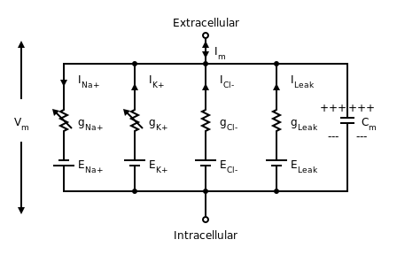 Membrane Circuit by Nrets, Source:
The capacitive current across the cell membrane can be described as the sum of changes in the membrane voltage \(V_m\) and ion currents caused primarily by sodium (Na) and potassium (K) and other leakages (L), mainly chloride ions. The ion currents are defined by their conductances (\(g\), with the Na and K conductances being voltage depended), their equilibrium potentials (\(E\)) and how the channel gates open and close (\(m, n, h\)): \[ \begin{align} I_{ext} &= C_m \frac{dV_m}{dt} + I_{ion}\\ & = C_m \frac{dV_m}{dt} + g_{Na} m^3 h(V-E_{Na}) + g_K n^4 (V - E_K) + g_L (V - E_L) \end{align} \]
The standard Hodgkin-Huxley model expands into a set of four differential equations: \[ \begin{align} C \frac{dV}{dt} & = I - g_{Na} m^3 h(V-E_{Na}) - g_K n^4 (V - E_K) -g_L (V - E_L)\\ \frac{dm}{dt} & = a_m(V) (1 - m) - b_m(V)m\\ \frac{dh}{dt} & = a_h(V)(1 - h) - b_h(V)h\\ \frac{dn}{dt} & = a_n(V) (1 - n) - b_n(V)n\\ a_m(V) & = 0.1(V+40)/(1 - \exp(-(V+40)/10))\\ b_m(V) & = 4 \exp(-(V + 65)/18)\\ a_h(V) & = 0.07 \exp(-(V+65)/20)\\ b_h(V) & = 1/(1 + \exp(- (V + 35)/10))\\ a_n(V) & = 0.01 (V + 55)/(1 - \exp(-(V+55)/10))\\ b_n(V) & = 0.125 \exp(-(V + 65)/80) \end{align} \]
To model and simulate those differential equations in R I use the simecol package. The package comes with a great vignette which gives a good introduction, and you may also find my recent LondonR talk helpful.
library(simecol)
## Hodkin-Huxley model
HH <- odeModel(
main = function(time, init, parms) {
  with(as.list(c(init, parms)),{

    am <- function(v) 0.1*(v+40)/(1-exp(-(v+40)/10))
    bm <- function(v) 4*exp(-(v+65)/18)
    ah <- function(v) 0.07*exp(-(v+65)/20)
    bh <- function(v) 1/(1+exp(-(v+35)/10))
    an <- function(v) 0.01*(v+55)/(1-exp(-(v+55)/10))
    bn <- function(v) 0.125*exp(-(v+65)/80)

    dv <- (I - gna*h*(v-Ena)*m^3-gk*(v-Ek)*n^4-gl*(v-El))/C
    dm <- am(v)*(1-m)-bm(v)*m
    dh <- ah(v)*(1-h)-bh(v)*h
    dn <- an(v)*(1-n)-bn(v)*n

    return(list(c(dv, dm, dh, dn)))
  })
  },
  ## Set parameters
  parms = c(Ena=50, Ek=-77, El=-54.4, gna=120, gk=36, gl=0.3, C=1, I=0),
  ## Set integrations times
  times = c(from=0, to=40, by = 0.25),
  ## Set initial state
  init = c(v=-65, m=0.052, h=0.596, n=0.317),
  solver = "lsoda"
)
Let’s run and plot the model:
HH <- sim(HH)
plot(HH) 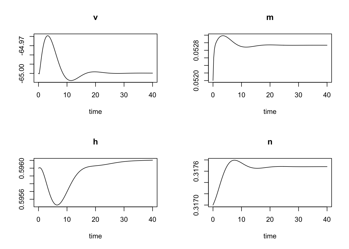
From the initial state I observe a tiny stimulus which reverts quickly back to the resting state. So let’s increase the external stimulus in steps to observe its impact on the membrane voltage:
times(HH)["to"] <- 100
## Stimulus
I <- c(2, 5, 5.97, 5.975, 6.2, 6.5)
sims <- do.call("rbind",
          lapply(I, function(i){
            parms(HH)["I"] <- i
            HH <- sim(HH)
            cbind(I=paste("I =", i), out(HH))
          }))
## Plot the various experiments with lattice
library(latticeExtra)
asTheEconomist(
  xyplot(v ~ time | factor(I), data=sims, type="l",
         as.table=TRUE,
         main="Hodgkin-Huxely model with varying external stimulus"),
xlab="time (ms)", ylab="mV")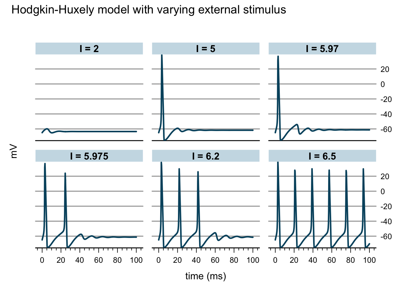
Now this is exciting, as I increase the external stimulus an action potential is generated. Increasing the stimulus further results in a constant firing of the neuron, or in other words, the model is going through a Hopf-bifurcation. I think it is absolutely remarkable what Hodgkin and Huxley achieved 60 years ago. They were able to demonstrate that numerical integration of their model could reproduce all the key biophysical properties of the action potential. And what seems so easy on a computer with R or other software, such as XPP/XPPAUT today, must have been a lot of work in the late 40s, early 50s of the 20th century.
Citation
For attribution, please cite this work as:Markus Gesmann (Jun 25, 2012) Hodgkin-Huxley model in R. Retrieved from https://magesblog.com/post/2012-06-25-hodgkin-huxley-model-in-r/
@misc{ 2012-hodgkin-huxley-model-in-r,
author = { Markus Gesmann },
title = { Hodgkin-Huxley model in R },
url = { https://magesblog.com/post/2012-06-25-hodgkin-huxley-model-in-r/ },
year = { 2012 }
updated = { Jun 25, 2012 }
}